import matplotlib
if not hasattr(matplotlib.RcParams, "_get"):
    matplotlib.RcParams._get = dict.get
16.2 Music understanding#
So far, we have studied how AI can generate music. The opposite direction, recognizing high-level semantic information in music, is the goal of music information retrieval (MIR), also called music understanding. Most often, the input is a recording, but MIR also works with symbolic music, and even images of sheet music:

Fig. 138 Music understanding recognizes many kinds of information in a recording, such as its genre, its tempo and key, its score, the separate recordings of its instruments (stems), and other music that sounds similar.#
Music classification#
Say you were asked to write a program that recognizes the genre of a recording. For example, given these two recordings, it should output “punk” for the first, and “jazz” for the second:
Excerpts of two clips from the FreeTZAN dataset. The Zombie Dandies - Red the Hunter, License: CC BY 4.0. Kevin MacLeod - I Knew a Guy, License: CC BY 3.0.
How would you do it? It’s not at all obvious how we would write down rules for this decision by hand. Perhaps the best that we can do is to learn to make it from data. This is the idea of supervised learning:
Definition 55 (Supervised learning)
Given training examples of inputs \(x\) paired with labels \(y\), supervised learning fits a model \(f_\theta\) to predict the label of each input, \(f_\theta(x) \approx y\), by minimizing a loss function that measures the difference between its predictions and the labels.
For example, \(x\) might be a recording and \(y\) its genre, such as “jazz” or “punk”. Notice the similarity to training a language model, where the “label” of each context is the next element. Once trained, the model can hopefully predict labels for new inputs that it has never seen.
Audio features#
What should we use as the input \(x\)? A thirty-second recording contains over a million samples, and individual samples are not very meaningful on their own. Instead, consider how you recognize genres. Recall from Chapter 15 that our inner ear decomposes sound into frequency bands, the critical bands. We perceive sound in the frequency domain, hearing the buzz of a distorted guitar or the shimmer of a cymbal, not individual samples. So it stands to reason that we should transform sound into similar features before classifying it.
MIR systems often use the spectrograms of Chapter 10 as features. A log-mel spectrogram goes a step further. Much like the critical bands, it groups the frequency bins of each frame into a few dozen bands that are evenly spaced on the mel scale, a perceptual scale of pitch. Then, much like our perception of loudness, it takes the logarithm of the energy in each band:
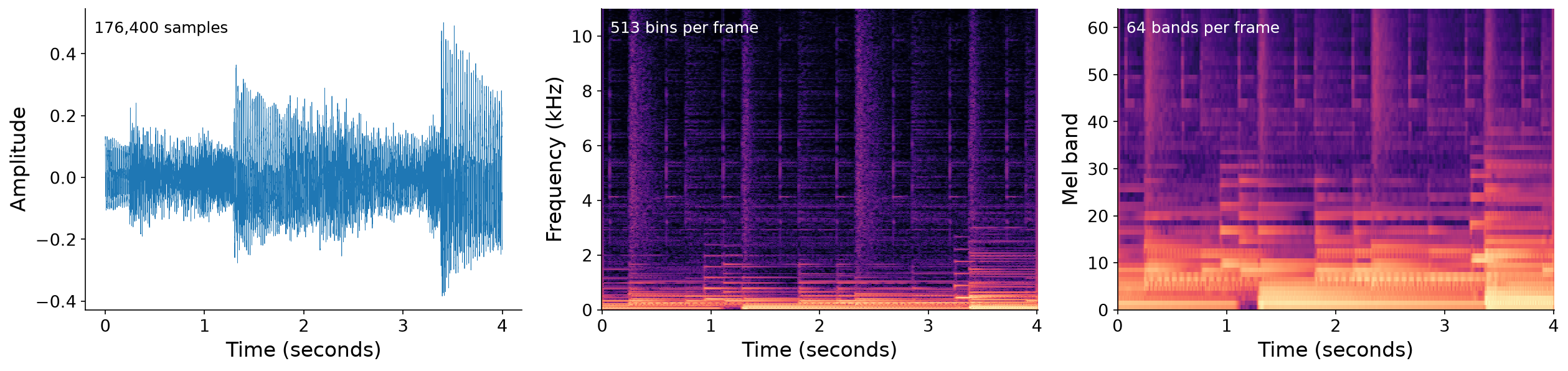
Fig. 139 The jazz trio from Chapter 10, as a waveform (left), a spectrogram (middle), and a log-mel spectrogram (right). Each is more compact, and closer to our perception, than the last.#
Example: genre classification. Let’s try this on FreeTZAN, a small, openly licensed dataset of thirty-second clips from the Free Music Archive [DBVB17], in \(10\) genres: ambient, classical, electronic, experimental, folk, hip-hop, jazz, pop, punk, and rock. We’ll use \(1000\) of its clips for training, and \(100\) others for evaluating accuracy, with no artist appearing in both. The labels are the genres that the artists chose for their own tracks, so they are noisy, and some clips are hard to classify even for a human listener.
The code below compares three kinds of features: (1) one second of the waveform, downsampled to \(1\) kHz, (2) the amplitude spectrogram, and (3) the log-mel spectrogram with \(64\) bands. To summarize each clip as a single vector, we average the spectrogram over time. The log-mel spectrogram is compact enough that we can afford two numbers per band: its average over time, and its standard deviation over time, which captures how much the band fluctuates (for example, with drum hits). (To fit the dataset into this book, these features were computed ahead of time.) For each kind of feature, the code trains a logistic regression classifier, one of the simplest models for classification:
data = np.load("./assets/freetzan-features.npz")   # features of FreeTZAN's clips
genre = data["genre"]                                # labels: 0 to 9, one per genre
train, test = data["split"] == "train", data["split"] == "test"

for name in ["waveform", "spectrogram", "log_mel"]:
    X = data[name].astype(np.float64)                # one row of features per clip
    predict = train_classifier(X[train], genre[train])   # learn from the 1000 training clips
    print(f"{name:11s} ({X.shape[1]:4d} features per clip): "
          f"train accuracy {np.mean(predict(X[train]) == genre[train]):4.0%}, "
          f"test accuracy {np.mean(predict(X[test]) == genre[test]):4.0%}")
waveform (1000 features per clip): train accuracy 97%, test accuracy 15%
spectrogram ( 513 features per clip): train accuracy  67%, test accuracy  36%
log_mel     ( 128 features per clip): train accuracy  56%, test accuracy  41%
Since the \(10\) genres are equally common, guessing at random would be right \(10\%\) of the time. The waveform does barely better than chance, at \(15\%\). The spectrogram does more than twice as well, at \(36\%\). The log-mel spectrogram does better still, at \(41\%\), with a quarter as many features as the spectrogram.
Overfitting. Notice that the waveform classifier is \(97\%\) accurate on its training clips, but only \(15\%\) accurate on the other clips. This is called overfitting, and it shows up as a gap between a model’s performance on its training data and on held-out data, data that it never saw during training. This is why we always evaluate models on held-out data.
Music transcription#
In Chapter 10, we transcribed a simple sine melody by taking the loudest frequency of each frame. Can’t we do the same for “real” music? Unfortunately, transcription is much more complicated than that. Real instruments produce harmonics (Chapter 3), so the loudest frequency may be a harmonic rather than the fundamental. And real music is polyphonic, with many notes from many instruments sounding at once, whose harmonics overlap:
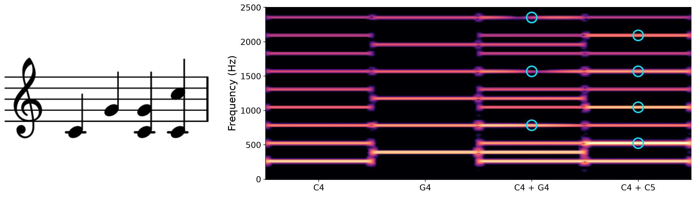
Fig. 140 A toy score (left) and the spectrogram of its additive synthesis (right), with \(10\) harmonics per note. Circles mark the harmonics shared by two notes. Every harmonic of C5 is also a harmonic of C4, so adding C5 to C4 adds no new frequencies at all.#
The code below tries two naive strategies on the jazz trio, neither of which should be expected to produce satisfactory results: (1) the loudest frequency of each frame, as in Chapter 10, and (2) treating every pitch whose energy is in the top \(K\%\) of a pitch-band spectrogram as a note:
# Strategy 1 (Chapter 10): the loudest frequency in each frame, rounded to the nearest pitch
audio = pq.Audio.from_file("./assets/audio-trio.wav")
pq.play(audio)                                            # what we are transcribing
N_F, N_H = 8192, 1024                                     # long frames: the bass notes are low
S, freqs = stft(audio, N_F, N_H)
loudest = np.round(frequency_to_pitch(freqs[np.argmax(S, axis=1)]))
loudest[S.max(axis=1) < 0.05 * S.max()] = -1             # too quiet: no pitch
pitches = np.arange(21, 109)                              # the 88 piano keys
on = loudest[:, None] == pitches                          # (num_frames, 88): at most one pitch on per frame
score = notes_from_frames(on, pitches, N_H / audio.sample_rate)   # a new note whenever the pitch changes
print(f"{len(score)} notes")
plot_transcriptions(S, freqs, N_H / audio.sample_rate, {"": score})
pq.play(sonify(score, audio))
18 notes

# Strategy 2: a pitch is on in a frame if its bin is among the loudest K% of all bins
P, pitches = pitch_spectrogram(S, freqs)                  # mel spectrogram, (num_frames, num_pitches)
scores = {}
for K in [1, 10]:
    on = P > np.percentile(P, 100 - K)                    # one global threshold for every bin
    score = notes_from_frames(on, pitches, N_H / audio.sample_rate)   # each run of "on" frames is a note
    print(f"K = {K}%: {len(score)} notes")
    scores[f"K = {K}%"] = score
plot_transcriptions(S, freqs, N_H / audio.sample_rate, scores)
for score in scores.values():
    pq.play(sonify(score, audio))
K = 1%: 18 notes
K = 10%: 132 notes

Neither strategy comes close to a faithful transcription. To transcribe real music, we need to train a model on recordings paired with the exact pitches and timings of their notes [HES+18]. The details are out of scope for this book, but the end of this chapter points to further reading.
Beyond classification and transcription#
We have only scratched the surface of music understanding. MIR studies many more tasks, such as tracking beats, recognizing chords, separating instruments, transcribing lyrics, and recommending music. But most of these tasks share a few common goals and techniques: (1) recognizing or predicting the underlying components of musical recordings, such as their notes, chords, beats, and instruments, (2) training neural networks on labeled data, and increasingly on large amounts of unlabeled data, and (3) evaluating and comparing methods on held-out data. The end of this chapter points to research on many of these tasks.