13.7 Spatial audio

13.7 Spatial audio#

Localization is our ability to perceive the direction and distance of a sound source. We rely on several cues to localize sound:

Time differences: a sound from our left reaches our left ear slightly before our right ear.
Level differences: our head blocks some of the sound on its way to the far ear, so a sound from our left is slightly louder in our left ear.
Spectral cues: our outer ears, the pinnae, filter sound differently depending on the direction it comes from, which helps us tell front from back and up from down.

Spatial audio aims to preserve or recreate these cues, so that listeners hear sounds coming from particular places.

Stereo#

The most common form of spatial audio is stereo, which records and plays back two channels of audio, for the left and the right. To record in stereo, we place two microphones apart from each other. A sound source closer to the left microphone reaches it earlier and louder than the right microphone, so the two channels capture the time and level differences between them. We store the two channels together as a matrix \(\mathbf{x} \in \mathbb{R}^{T f_s \times 2}\), for \(T\) seconds of audio at sample rate \(f_s\), or in Pyquist, as an pq.Audio whose pq.Audio.num_channels is \(2\). Finally, we play back the two channels over two loudspeakers, or a pair of headphones, which recreates the cues for the listener:

A diagram in three panels. Left, recording: a gold sound source emits wavefronts toward two microphones, labeled L and R, and the source is closer to the left microphone. Middle, storage: two waveforms, labeled L and R, show the same pulse, which arrives later and smaller in the R channel, above the label x in R to the T f_s by 2. Right, playback: two loudspeakers, labeled L and R, emit wavefronts toward a listener's head below them. 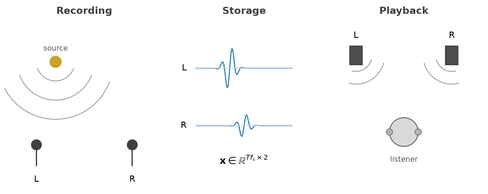— Fig. 109 Stereo recording (left), storage (middle), and playback (right). The sound reaches the left microphone first, and more loudly, so the left channel leads the right channel.#

Panning#

What if we have a mono recording, but want it to sound as if it comes from a particular direction? We can simulate a level difference by sending the sound to the two channels with different gains, which is called panning. With a pan position \(\alpha\) from \(0\) (left) to \(1\) (right), the simplest approach is linear panning:

\[x_L[n] = (1 - \alpha) \cdot x[n], \qquad x_R[n] = \alpha \cdot x[n].\]

But linear panning has a subtle flaw. When two loudspeakers play the same sound, its loudness depends roughly on the sum of the squares of the two channels’ gains, rather than the sum of the gains. At the center, \(\alpha = \frac{1}{2}\), the squared gains sum to only \((\frac{1}{2})^2 + (\frac{1}{2})^2 = \frac{1}{2}\). So with linear panning, a sound seems to get quieter as it passes through the middle, a “hole in the middle”. Constant-power panning (so named because the power of a sound is proportional to its squared amplitude) avoids this problem by using a quarter cycle of a cosine and a sine:

\[x_L[n] = \cos\left(\frac{\alpha \pi}{2}\right) \cdot x[n], \qquad x_R[n] = \sin\left(\frac{\alpha \pi}{2}\right) \cdot x[n].\]

Since \(\cos^2 \theta + \sin^2 \theta = 1\), the squared gains sum to \(1\) at every position:

Two plots of channel gain versus pan position alpha from 0 to 1. Left, linear panning: the left gain falls in a straight line from 1 to 0, the right gain rises in a straight line from 0 to 1, and they cross at 0.5. The dashed sum of the squared gains dips from 1 at the edges to 0.5 at the center. Right, constant-power panning: the left gain follows a quarter cosine and the right gain a quarter sine, crossing at 0.707, and the dashed sum of the squared gains stays flat at 1. 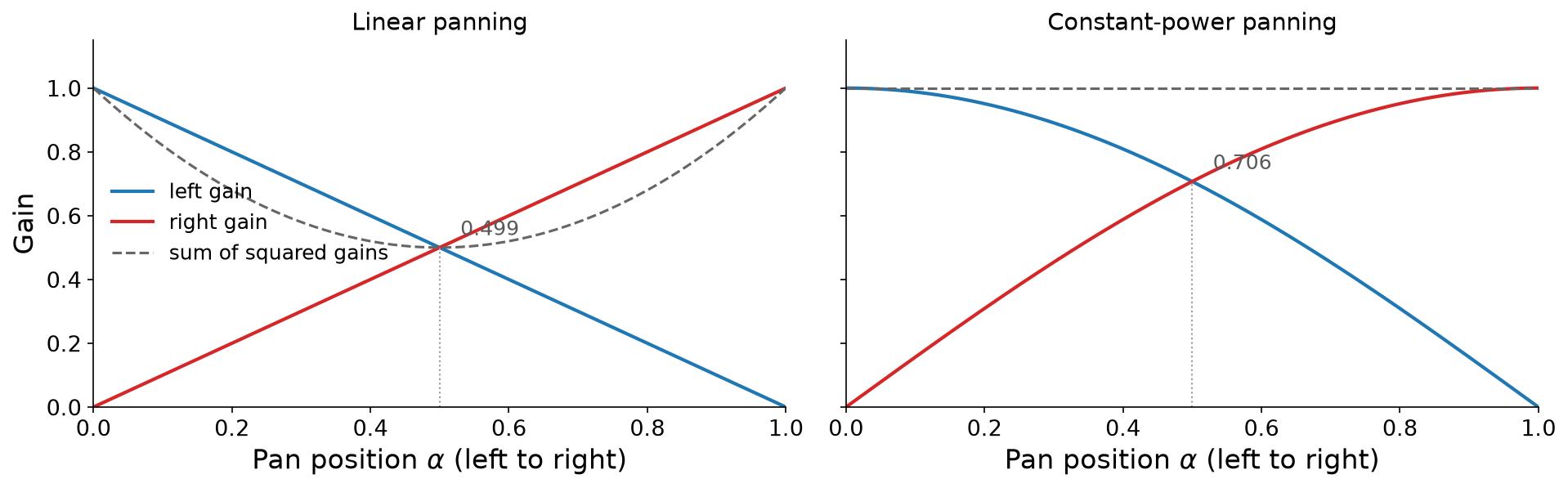— Fig. 110 Linear panning (left) and constant-power panning (right). The dashed lines show the sum of the squared gains of the two channels.#

Pyquist implements constant-power panning in pq.Audio.pan, with a position from \(-1\) (left) to \(1\) (right), which corresponds to \(\alpha\) from \(0\) to \(1\). The code below plays a marimba five times, moving it from left to right, by rendering a pq.Score whose events specify a pan position. Listen with headphones:

# hide
import pyquist as pq

marimba = pq.Audio.from_file("./assets/marimba.wav").segment(offset=0.5, duration=2.0)


def panned_marimba(position: float) -> pq.Audio:
    """The marimba, panned to `position`, from -1 (left) to 1 (right)."""
    return marimba.as_stereo().pan(position, in_place=False)


score = pq.Score([(2.0 * i, {"position": p}) for i, p in enumerate([-1.0, -0.5, 0.0, 0.5, 1.0])])
pq.play(score.render(panned_marimba), normalize=True)

Ping-pong delay#

Spatial audio combines naturally with feedback delay lines. A ping-pong delay is a stereo feedback delay whose echoes bounce back and forth between the left and right channels. It uses two delay lines, one per channel, each of which feeds back into the other channel. The code below applies a ping-pong delay to the sound of a single bounce of a ping-pong ball:

# hide
import numpy as np
import pyquist as pq

def ping_pong_delay(x: np.ndarray, M: int, g: float) -> np.ndarray:
    """A stereo feedback delay whose echoes bounce between the left and right channels."""
    left_buffer, right_buffer = np.zeros(M), np.zeros(M)   # two delay lines
    i = 0
    y = np.zeros((len(x), 2))
    for n in range(len(x)):
        y[n, 0] = x[n] + g * right_buffer[i]   # echoes from the right return on the left
        y[n, 1] = g * left_buffer[i]           # echoes from the left return on the right
        left_buffer[i], right_buffer[i] = y[n, 0], y[n, 1]
        i = (i + 1) % M
    return y


ball = pq.Audio.from_file("./assets/ping-pong.wav")
f_s = ball.sample_rate
hit = ball.segment(offset=0.5, duration=0.3).samples[:, 0]   # a single bounce
x = np.concatenate([hit, np.zeros(3 * f_s)])                 # room for the echoes
pq.play(pq.Audio(ping_pong_delay(x, M=round(0.3 * f_s), g=0.7), f_s), normalize=True)

Sound from Freesound: 149732 by beskhu, License: Attribution 4.0.

Widening#

The width of a stereo sound is how much of the space between the loudspeakers it seems to occupy. To control width, we convert the left and right channels into a mid/side representation:

\[x_M[n] = x_L[n] + x_R[n], \qquad x_S[n] = x_L[n] - x_R[n].\]

The mid signal \(x_M\) contains what the two channels share, and the side signal \(x_S\) contains what differs between them. To widen a sound, we boost the side signal relative to the mid signal. To narrow it, we do the opposite. Then we convert back to left and right:

\[x_L[n] = \frac{x_M[n] + x_S[n]}{2}, \qquad x_R[n] = \frac{x_M[n] - x_S[n]}{2}.\]

The code below adjusts the width of a stereo synthesizer pad, by scaling its side signal by a width of (1) \(0\), which collapses the pad to mono, (2) \(1\), which leaves it unchanged, and (3) \(2\), which makes it wider. Again, listen with headphones:

# hide
import numpy as np
import pyquist as pq

pad = pq.Audio.from_file("./assets/pad-stereo.wav")
left, right = pad.samples[:, 0], pad.samples[:, 1]
mid, side = left + right, left - right
for width in [0.0, 1.0, 2.0]:                 # mono, unchanged, and wider
    widened = np.stack([(mid + width * side) / 2, (mid - width * side) / 2], axis=1)
    pq.play(pq.Audio(widened, pad.sample_rate), normalize=True)

Sound from Freesound: 37746 by Quilt, License: CC0.

Beyond stereo#

The stereo techniques we have discussed here cannot place sounds above, below, or behind the listener. One straightforward solution is to add more microphones, channels, and loudspeakers, as in surround sound. More sophisticated approaches like ambisonics and wave field synthesis represent the sound field itself, independently of any particular arrangement of loudspeakers. And for listeners with just a pair of headphones, binaural audio filters each sound with a head-related transfer function (HRTF), which simulates the time differences, level differences, and spectral cues of a particular direction.