import matplotlib
if not hasattr(matplotlib.RcParams, "_get"):
    matplotlib.RcParams._get = dict.get

14.1 n-gram statistics

In the previous section, we saw that we can use probabilities and stochastic processes to generate scores. But can we go the other way, and use scores to induce stochastic processes? Let’s build up some intuition for this question with a running example from Chapter 4, the first phrase of Twinkle, Twinkle, Little Star:

Fig. 113 The first phrase of Twinkle, Twinkle, Little Star, with the name and MIDI pitch of each note.

As a pq.Score, with times in beats, and leaving out durations for simplicity:

twinkle = pq.Score([
    (0, {"pitch": 60}),
    (1, {"pitch": 60}),
    (2, {"pitch": 67}),
    (3, {"pitch": 67}),
    (4, {"pitch": 69}),
    (5, {"pitch": 69}),
    (6, {"pitch": 67}),
])

Consider a stochastic process with \(N = 7\) notes, in which every \(X_i\) has the same alphabet of six pitches, \(\mathcal{X} = \{60, 62, 64, 65, 67, 69\}\) (C, D, E, F, G, and A), and the same uniform distribution, \(P(X_i = x) = \frac{1}{6}\). What is the likelihood of our melody, the probability that running this process generates it? In this process, each note is drawn independently of the others, so the probability of the whole sequence is the product of the probabilities of its notes:

\[ P(X_1 = 60) \cdot P(X_2 = 60) \cdot P(X_3 = 67) \cdot \ldots \cdot P(X_7 = 67) = \left(\frac{1}{6}\right)^7 = \frac{1}{279{,}936}. \]

We would expect to run this process \(279{,}936\) times before it generates our melody even once.

What happens if we change the stochastic process? Suppose that we instead use the alphabet \(\mathcal{X} = \{60, 67, 69\}\), just the three pitches of our melody, each with probability \(\frac{1}{3}\). Now the likelihood of our melody is \(\left(\frac{1}{3}\right)^7 = \frac{1}{2187}\), which is \(\frac{279{,}936}{2187} = 128\) times more likely than before. By modifying the process to better reflect the “data”, we improve the likelihood that it generates the sequences we are interested in.

Unigrams

How might we modify our process to be even more likely to generate our melody? Specifically, what alphabet and probabilities would maximize the likelihood of the melody?

Intuitively, the probabilities that maximize the likelihood of a sequence are exactly the ones that reflect its statistics. Our alphabet should contain only the pitches of the sequence, and the probability of each pitch should be the fraction of the sequence that it makes up. This gives us a new stochastic process. Like our first one, it draws each of the \(N\) notes independently, from the same distribution, but now that distribution reflects the melody:

\[P(X_i = x) = \frac{\text{count}(x)}{N} \quad \text{for all } i.\]

The first phrase of Twinkle, Twinkle, Little Star (C C G G A A G, or \(60, 60, 67, 67, 69, 69, 67\)) contains \(60\) twice, \(67\) three times, and \(69\) twice. So \(P(X_i = 60) = \frac{2}{7}\), \(P(X_i = 67) = \frac{3}{7}\), and \(P(X_i = 69) = \frac{2}{7}\), and the likelihood of the melody is now

\[\frac{2}{7} \cdot \frac{2}{7} \cdot \frac{3}{7} \cdot \frac{3}{7} \cdot \frac{2}{7} \cdot \frac{2}{7} \cdot \frac{3}{7} = \frac{432}{823{,}543} \approx \frac{1}{1906}.\]

For a process that draws every note independently from the same distribution, this is the best we can do (we have maximized the likelihood). This basic strategy, counting how often each outcome occurs to model a sequence of outcomes, is known as a unigram model, for reasons that will become clear shortly. The code below fits a unigram model to our melody by counting, and generates seven notes from it. The generated melodies have pitches in the right proportions, but in a random order:

# hide
import numpy as np
import pyquist as pq
from scipy.signal import lfilter

# hide
def pluck(pitch: float, duration: float, f_s: int = 44100, **kwargs) -> pq.Audio:
    """A Karplus-Strong plucked string (Chapter 12) that decays by 60 dB in `duration`
    seconds. An all-pass filter (Chapter 13) in the loop tunes it precisely."""
    P = f_s / pq.helper.pitch_to_frequency(pitch)   # the period, in (fractional) samples
    M = int(P - 0.6)                                 # the delay line (the low-pass adds 1/2 sample)
    D = P - 0.5 - M                                  # the all-pass adds the remaining D samples
    c = (1 - D) / (1 + D)                            # the all-pass gain for a delay of D samples
    g = 10 ** (-3 * P / (f_s * duration))            # decay by 60 dB over the duration
    x = np.zeros(int(duration * f_s))
    x[:M] = np.random.uniform(-1.0, 1.0, M)          # excitation: a burst of white noise
    # The whole loop is one recursive filter (Chapter 9), which SciPy runs quickly:
    # y[n] = x[n] + c x[n-1] - c y[n-1] + (g/2) (c y[n-M] + (1 + c) y[n-M-1] + y[n-M-2])
    a = np.zeros(M + 3)
    a[:2] = [1.0, c]
    a[M:] -= 0.5 * g * np.array([c, 1 + c, 1.0])
    return pq.Audio(lfilter([1.0, c], a, x), f_s)

def compute_unigram(melody: list[int]) -> tuple[list[int], np.ndarray]:
    """The states (pitches) of a melody, and the fraction of the melody each one makes up."""
    states = sorted(set(melody))
    counts = np.array([melody.count(pitch) for pitch in states])
    return states, counts / len(melody)


def unigram(N: int, states: list[int], probabilities: np.ndarray, ioi: float = 1.0,
            duration: float = 1.0) -> pq.Score:
    """A melody of N notes, each drawn independently from the unigram probabilities.
    Onsets are in beats, and durations (decay times) are in seconds."""
    choices = np.random.choice(states, size=N, p=probabilities)
    return pq.Score([(i * ioi, {"pitch": int(pitch), "duration": duration})
                     for i, pitch in enumerate(choices)])


melody = [60, 60, 67, 67, 69, 69, 67]           # Twinkle, Twinkle, Little Star
states, probabilities = compute_unigram(melody)
print(states, probabilities)

score = unigram(7, states, probabilities)
print([kwargs["pitch"] for _, kwargs in score])
pq.play(score.render(pluck, metronome=pq.BasicMetronome(bpm=120)), normalize=True)

[60, 67, 69] [0.28571429 0.42857143 0.28571429]
[60, 60, 67, 60, 60, 67, 67]

Markov chains

In a unigram model, every position has the same probabilities, and each choice is independent of the others: knowing the previous note tells us nothing about the next one. This assumption is unwieldy for music, where notes relate to one another in time. For example, in many melodies, each note tends to be close in pitch to the note before it. To capture relationships like this, we need the notion of conditional probability:

Definition 44 (Conditional probability)

The conditional probability \(P(X = x \mid Y = y)\) is the probability that a random variable \(X\) takes the value \(x\), given that we know that a random variable \(Y\) took the value \(y\). For each value \(y\), it is a categorical distribution over the outcomes of \(X\).

If \(P(X = x \mid Y = y) = P(X = x)\) for all \(x\) and \(y\), then knowing \(Y\) tells us nothing about \(X\), and we say that \(X\) and \(Y\) are independent.

With conditional probability in hand, we can define a stochastic process whose outcomes depend on one another:

Definition 45 (Markov chain)

A Markov chain is a stochastic process in which the distribution of each outcome depends on the previous outcome. It consists of (1) a set of states, its alphabet \(\mathcal{X}\), and (2) the transition probabilities \(P(X_i = b \mid X_{i-1} = a)\) of moving from each state \(a\) to each state \(b\).

We can draw a Markov chain as a graph, with a node for each state and an arrow for each transition, labeled with its probability. We can also write its transition probabilities as a transition matrix \(T \in [0, 1]^{|\mathcal{X}| \times |\mathcal{X}|}\) (the weighted adjacency matrix of the graph), whose rows are previous states, and whose columns are next states:

\[T_{a, b} = P(X_i = b \mid X_{i-1} = a).\]

For example, here is a Markov chain with two states, the notes C and G. When the previous note is C, the next note is C with probability \(\frac{1}{3}\), and G with probability \(\frac{2}{3}\). When the previous note is G, the next note is always C:

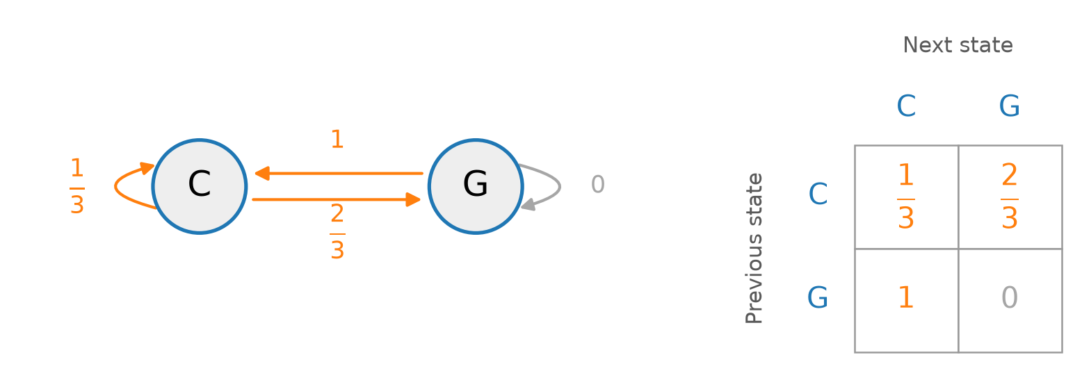
Fig. 114 A Markov chain with two states, drawn as a graph (left), and as a transition matrix (right). Rows are previous states, and columns are next states.

Each row of the transition matrix is a categorical distribution over the next state, so it sums to one: \(\sum_{b \in \mathcal{X}} T_{a, b} = 1\) for every state \(a\).

The Markov chain is the first stochastic process we have studied whose behavior depends on context: the probabilities of each note depend on the note before it. But how much context does it use? Only the previous state. Given \(X_{i-1}\), a Markov chain assumes that the next state \(X_i\) is independent of all of the states before it, \(X_1, \ldots, X_{i-2}\):

\[P(x_i \mid x_1, \ldots, x_{i-1}) = P(x_i \mid x_{i-1}).\]

This is called the Markov assumption.

To generate from a Markov chain, we draw the first state from some distribution, for example, uniformly at random. Then we repeatedly draw the next state from the row of the transition matrix for the current state, \(x_i \sim P(X_i \mid X_{i-1} = x_{i-1})\). The animation below shows this process for a Markov chain with three states, C, G, and A. At each step, the transitions out of the current state light up, one of them is drawn at random, and the new state joins the generated sequence, along with its probability:

The code below implements this process, for a Markov chain whose \(12\) states are the white keys of a piano from C4 to G5. Rather than learning its transition probabilities from data, we engineered them by hand, using some basic musical knowledge. Melodies tend to move to a neighboring note, sometimes jump a little further, and B tends to move up to C. Notice how sparse the transition matrix is: most of its entries are zero.

# hide
import numpy as np
import pyquist as pq
from scipy.signal import lfilter

# hide
def pluck(pitch: float, duration: float, f_s: int = 44100, **kwargs) -> pq.Audio:
    """A Karplus-Strong plucked string (Chapter 12) that decays by 60 dB in `duration`
    seconds. An all-pass filter (Chapter 13) in the loop tunes it precisely."""
    P = f_s / pq.helper.pitch_to_frequency(pitch)   # the period, in (fractional) samples
    M = int(P - 0.6)                                 # the delay line (the low-pass adds 1/2 sample)
    D = P - 0.5 - M                                  # the all-pass adds the remaining D samples
    c = (1 - D) / (1 + D)                            # the all-pass gain for a delay of D samples
    g = 10 ** (-3 * P / (f_s * duration))            # decay by 60 dB over the duration
    x = np.zeros(int(duration * f_s))
    x[:M] = np.random.uniform(-1.0, 1.0, M)          # excitation: a burst of white noise
    # The whole loop is one recursive filter (Chapter 9), which SciPy runs quickly:
    # y[n] = x[n] + c x[n-1] - c y[n-1] + (g/2) (c y[n-M] + (1 + c) y[n-M-1] + y[n-M-2])
    a = np.zeros(M + 3)
    a[:2] = [1.0, c]
    a[M:] -= 0.5 * g * np.array([c, 1 + c, 1.0])
    return pq.Audio(lfilter([1.0, c], a, x), f_s)

def markov(N: int, states: list[int], initial_state: int | None, probabilities: np.ndarray,
           ioi: float = 0.5, duration: float = 0.5) -> pq.Score:
    """A melody of N notes from a Markov chain. Row a of `probabilities` is the
    distribution of the next state, given that the previous state is states[a].
    Onsets are in beats, and durations (decay times) are in seconds."""
    if initial_state is None:
        a = np.random.randint(len(states))           # the first state, uniformly at random
    else:
        a = states.index(initial_state)
    events = []
    for i in range(N):
        events.append((i * ioi, {"pitch": states[a], "duration": duration}))
        a = np.random.choice(len(states), p=probabilities[a])   # transition to the next state
    return pq.Score(events)


#         C4  D4  E4  F4  G4  A4  B4  C5  D5  E5  F5  G5
states = [60, 62, 64, 65, 67, 69, 71, 72, 74, 76, 77, 79]
probabilities = np.array([
    # C4   D4   E4   F4   G4   A4   B4   C5   D5   E5   F5   G5
    [0.0, 0.4, 0.3, 0.0, 0.2, 0.0, 0.0, 0.1, 0.0, 0.0, 0.0, 0.0],  # from C4
    [0.4, 0.0, 0.4, 0.1, 0.1, 0.0, 0.0, 0.0, 0.0, 0.0, 0.0, 0.0],  # from D4
    [0.2, 0.3, 0.0, 0.3, 0.2, 0.0, 0.0, 0.0, 0.0, 0.0, 0.0, 0.0],  # from E4
    [0.0, 0.1, 0.5, 0.0, 0.3, 0.1, 0.0, 0.0, 0.0, 0.0, 0.0, 0.0],  # from F4
    [0.0, 0.0, 0.2, 0.2, 0.1, 0.3, 0.0, 0.2, 0.0, 0.0, 0.0, 0.0],  # from G4
    [0.0, 0.0, 0.0, 0.1, 0.4, 0.0, 0.3, 0.2, 0.0, 0.0, 0.0, 0.0],  # from A4
    [0.0, 0.0, 0.0, 0.0, 0.1, 0.2, 0.0, 0.7, 0.0, 0.0, 0.0, 0.0],  # from B4
    [0.0, 0.0, 0.0, 0.0, 0.2, 0.0, 0.3, 0.1, 0.3, 0.1, 0.0, 0.0],  # from C5
    [0.0, 0.0, 0.0, 0.0, 0.0, 0.0, 0.1, 0.4, 0.0, 0.4, 0.1, 0.0],  # from D5
    [0.0, 0.0, 0.0, 0.0, 0.0, 0.0, 0.0, 0.2, 0.3, 0.0, 0.3, 0.2],  # from E5
    [0.0, 0.0, 0.0, 0.0, 0.0, 0.0, 0.0, 0.0, 0.2, 0.6, 0.0, 0.2],  # from F5
    [0.0, 0.0, 0.0, 0.0, 0.2, 0.0, 0.0, 0.2, 0.0, 0.3, 0.3, 0.0],  # from G5
])
assert np.allclose(probabilities.sum(axis=1), 1.0)   # each row is a distribution

score = markov(32, states, None, probabilities)
pq.play(score.render(pluck, metronome=pq.BasicMetronome(bpm=120)), normalize=True)

Fitting Markov chains to data

How should we set the transition probabilities of a Markov chain, to maximize the likelihood of a particular sequence? As for unigrams, the answer is to count. The transition probabilities that maximize the likelihood of a sequence are

\[P(X_i = b \mid X_{i-1} = a) = \frac{\text{count}(a \to b)}{\text{count}(a \to \cdot)},\]

where \(\text{count}(a \to b)\) is the number of times that state \(a\) is immediately followed by state \(b\), and \(\text{count}(a \to \cdot) = \sum_{b' \in \mathcal{X}} \text{count}(a \to b')\) is the number of times that \(a\) is followed by any state.

Let’s fit a Markov chain to the first phrase of Twinkle, Twinkle, Little Star, C C G G A A G. Its states are C, G, and A (\(60\), \(67\), and \(69\)), and it contains six transitions: C → C, C → G, G → G, G → A, A → A, and A → G. (The final G has no next note, so it does not count.) Each state is followed by two different states, once each. So every transition that occurs has probability \(\frac{1}{2}\), and every other transition has probability \(0\):

Fig. 115 The Markov chain that maximizes the likelihood of the first phrase of Twinkle, Twinkle, Little Star, drawn as a graph (left, with transitions of probability \(0\) in gray), and as a transition matrix (right).

How should we choose the probability of the first note, \(P(X_1)\)? There are at least three options: (1) a uniform distribution, \(P(X_1 = 60) = \frac{1}{|\mathcal{X}|} = \frac{1}{3}\), (2) the unigram probability, \(P(X_1 = 60) = \frac{2}{7}\), or (3) always starting on the first note of the melody, \(P(X_1 = 60) = 1\). Let’s go with the third option. Then the likelihood of the melody is the probability of its first note, times the probability of each of its transitions:

\[P(X_1 = 60) \cdot P(X_2 = 60 \mid X_1 = 60) \cdot \ldots \cdot P(X_7 = 67 \mid X_6 = 69) = 1 \cdot \left(\frac{1}{2}\right)^6 = \frac{1}{64}.\]

That is about \(30\) times more likely than under the unigram model (\(\approx \frac{1}{1906}\)). The code below fits this Markov chain by counting transitions, and generates melodies from it. The melodies mix and match pieces of the original, but once they leave C, they never return, since no transition leads back to it.

# hide
import numpy as np
import pyquist as pq
from scipy.signal import lfilter

# hide
def pluck(pitch: float, duration: float, f_s: int = 44100, **kwargs) -> pq.Audio:
    """A Karplus-Strong plucked string (Chapter 12) that decays by 60 dB in `duration`
    seconds. An all-pass filter (Chapter 13) in the loop tunes it precisely."""
    P = f_s / pq.helper.pitch_to_frequency(pitch)   # the period, in (fractional) samples
    M = int(P - 0.6)                                 # the delay line (the low-pass adds 1/2 sample)
    D = P - 0.5 - M                                  # the all-pass adds the remaining D samples
    c = (1 - D) / (1 + D)                            # the all-pass gain for a delay of D samples
    g = 10 ** (-3 * P / (f_s * duration))            # decay by 60 dB over the duration
    x = np.zeros(int(duration * f_s))
    x[:M] = np.random.uniform(-1.0, 1.0, M)          # excitation: a burst of white noise
    # The whole loop is one recursive filter (Chapter 9), which SciPy runs quickly:
    # y[n] = x[n] + c x[n-1] - c y[n-1] + (g/2) (c y[n-M] + (1 + c) y[n-M-1] + y[n-M-2])
    a = np.zeros(M + 3)
    a[:2] = [1.0, c]
    a[M:] -= 0.5 * g * np.array([c, 1 + c, 1.0])
    return pq.Audio(lfilter([1.0, c], a, x), f_s)

def markov(N: int, states: list[int], initial_state: int | None, probabilities: np.ndarray,
           ioi: float = 0.5, duration: float = 0.5) -> pq.Score:
    """A melody of N notes from a Markov chain. Row a of `probabilities` is the
    distribution of the next state, given that the previous state is states[a].
    Onsets are in beats, and durations (decay times) are in seconds."""
    if initial_state is None:
        a = np.random.randint(len(states))           # the first state, uniformly at random
    else:
        a = states.index(initial_state)
    events = []
    for i in range(N):
        events.append((i * ioi, {"pitch": states[a], "duration": duration}))
        a = np.random.choice(len(states), p=probabilities[a])   # transition to the next state
    return pq.Score(events)

melody = [60, 60, 67, 67, 69, 69, 67]           # Twinkle, Twinkle, Little Star
states = sorted(set(melody))                    # [60, 67, 69]
counts = np.zeros((len(states), len(states)))
for a, b in zip(melody[:-1], melody[1:]):       # every transition a -> b in the melody
    counts[states.index(a), states.index(b)] += 1
probabilities = counts / counts.sum(axis=1, keepdims=True)
print(probabilities)

initial_state = 60
score = markov(16, states, initial_state, probabilities)
pq.play(score.render(pluck, metronome=pq.BasicMetronome(bpm=120)), normalize=True)

[[0.5 0.5 0. ]
 [0.  0.5 0.5]
 [0.  0.5 0.5]]

n-grams

In music, we know intuitively that notes depend on more than just the note immediately before them. For example, a melody that climbs C D E is likely to continue up to F, while a melody that falls G F E is likely to continue down to D, even though both just played E. How can we generalize Markov chains to longer contexts? First, we need a tool for computing the probability of a whole sequence:

Definition 46 (Chain rule of probability)

The probability that two random variables take the values \(x\) and \(y\) is the probability of the first, times the probability of the second given the first:

\[P(x, y) = P(x) \cdot P(y \mid x).\]

Applying this rule repeatedly, the probability of a sequence \(x_1, \ldots, x_N\) is

\[\begin{split} \begin{aligned} P(x_1, \ldots, x_N) &= P(x_1) \cdot P(x_2 \mid x_1) \cdot P(x_3 \mid x_1, x_2) \cdot \ldots \cdot P(x_N \mid x_1, \ldots, x_{N-1}) \\ &= \prod_{i=1}^{N} P(x_i \mid x_1, \ldots, x_{i-1}), \end{aligned} \end{split}\]

where the first factor (\(i = 1\)) has no condition, so it is just \(P(x_1)\).

The chain rule is exact: it makes no assumptions about the process. The models we have studied each simplify its factors. A unigram model ignores the context entirely, using \(P(x_i)\) for each factor. A Markov chain keeps only the previous state, \(P(x_i \mid x_{i-1})\), which is why its likelihood is the probability of its first state, times the probability of each transition.

An n-gram model keeps the previous \(n - 1\) states. Given these \(n - 1\) states, it assumes that \(X_i\) is independent of all earlier states:

\[P(x_i \mid x_1, \ldots, x_{i-1}) = P(x_i \mid x_{i-n+1}, \ldots, x_{i-1}).\]

Be careful to distinguish \(n\), the length of the context plus one, from \(N\), the length of the sequence.

Its name comes from n-grams, subsequences of \(n\) consecutive states. Once again, the probabilities that maximize the likelihood of a sequence come from counting:

\[P(b \mid a_1, \ldots, a_{n-1}) = \frac{\text{count}(a_1, \ldots, a_{n-1}, b)}{\text{count}(a_1, \ldots, a_{n-1}, \cdot)},\]

where \(\text{count}(a_1, \ldots, a_{n-1}, b)\) is the number of times the \(n\)-gram \((a_1, \ldots, a_{n-1}, b)\) occurs in the sequence, and the denominator is the number of times its context \((a_1, \ldots, a_{n-1})\) is followed by any state.

The models we have seen are special cases. A unigram model is an \(n\)-gram model with \(n = 1\) (no context at all), and a Markov chain has \(n = 2\), which is why it is also called a bigram model. With \(n = 3\), we have a trigram model, and so on.

Longer contexts come at a steep price. An \(n\)-gram model needs a probability for every possible context of \(n - 1\) states, followed by every possible next state, for a total of \(|\mathcal{X}|^n\) probabilities. This blows up very quickly. For example, a Markov chain over the \(88\) keys of a piano has \(88^2 = 7744\) probabilities, but a trigram model has \(88^3 = 681{,}472\).

This is an instance of the curse of dimensionality. Modern AI language models are based on the same basic idea as \(n\)-gram models, predicting what comes next from its context. A key distinction is that they have mechanisms to overcome the curse of dimensionality, such as recognizing that similar contexts should lead to similar predictions.

Meanwhile, the amount of data stays the same. A sequence of \(N\) states contains just \(N - n + 1\) \(n\)-grams, so as \(n\) grows, more and more of the probabilities are zero. The table gets sparser. For example, here are the bigram and trigram counts for all six phrases of Twinkle, Twinkle, Little Star (\(N = 42\) notes). Just \(14\) of the \(36\) bigram counts (\(38.9\%\)) are nonzero, and just \(18\) of the \(216\) trigram counts (\(8.3\%\)):

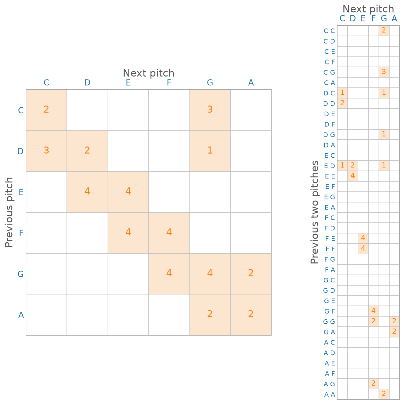
Fig. 116 Bigram counts (left) and trigram counts (right) for all of Twinkle, Twinkle, Little Star. Shaded cells are nonzero.

So we need to find a “Goldilocks” value of \(n\). With \(n = 1\), the model has no context at all. With \(n = N\), the model has seen just one context, the first \(N - 1\) states, so all it can do is copy the original sequence. More generally, as \(n\) grows, an \(n\)-gram model copies longer and longer passages of the sequence it was fit to. In practice, \(n = 2\) and \(n = 3\) are often the sweet spots between no context and copying.

In 1957, Brooks, Hopkins, Neumann, and Wright fit \(n\)-gram models with up to \(n = 8\) to a collection of \(37\) melodies, and generated new melodies from them [BHNW57], an early example of the techniques in this section.

The code below fits \(n\)-gram models to the melodies of three pieces, stored as MIDI files: all of Twinkle, Twinkle, Little Star, the first prelude of Bach’s The Well-Tempered Clavier, and Koji Kondo’s theme for Super Mario Bros. When a piece plays several notes at once, we keep only the highest. Along with the probabilities, compute_ngram measures the median IOI and the median duration of each melody, in seconds, so that the generated melodies move at about the same pace as the originals:

# hide
import numpy as np
import pyquist as pq
from scipy.signal import lfilter

# hide
def pluck(pitch: float, duration: float, f_s: int = 44100, **kwargs) -> pq.Audio:
    """A Karplus-Strong plucked string (Chapter 12) that decays by 60 dB in `duration`
    seconds. An all-pass filter (Chapter 13) in the loop tunes it precisely."""
    P = f_s / pq.helper.pitch_to_frequency(pitch)   # the period, in (fractional) samples
    M = int(P - 0.6)                                 # the delay line (the low-pass adds 1/2 sample)
    D = P - 0.5 - M                                  # the all-pass adds the remaining D samples
    c = (1 - D) / (1 + D)                            # the all-pass gain for a delay of D samples
    g = 10 ** (-3 * P / (f_s * duration))            # decay by 60 dB over the duration
    x = np.zeros(int(duration * f_s))
    x[:M] = np.random.uniform(-1.0, 1.0, M)          # excitation: a burst of white noise
    # The whole loop is one recursive filter (Chapter 9), which SciPy runs quickly:
    # y[n] = x[n] + c x[n-1] - c y[n-1] + (g/2) (c y[n-M] + (1 + c) y[n-M-1] + y[n-M-2])
    a = np.zeros(M + 3)
    a[:2] = [1.0, c]
    a[M:] -= 0.5 * g * np.array([c, 1 + c, 1.0])
    return pq.Audio(lfilter([1.0, c], a, x), f_s)

def compute_ngram(midi_path: str, n: int) -> tuple[list[int], np.ndarray, float, float]:
    """The states (pitches) of the melody of a MIDI file, its n-gram probabilities, and
    its median IOI and duration (in seconds). probabilities[a_1, ..., a_{n-1}, b] is the
    probability that states[b] follows the context states[a_1], ..., states[a_{n-1}]."""
    score, metronome = pq.Score.from_midi(midi_path)
    highest = {}                                 # the melody: the highest note at each onset
    for time, kwargs in score:
        if time not in highest or kwargs["pitch"] > highest[time]["pitch"]:
            highest[time] = kwargs
    onsets = sorted(highest)
    melody = [highest[time]["pitch"] for time in onsets]
    seconds = [metronome.tick_to_seconds(time) for time in onsets]
    ioi = float(np.median(np.diff(seconds)))
    duration = float(np.median([highest[time]["duration"] for time in onsets]))
    states = sorted(set(melody))
    indices = [states.index(pitch) for pitch in melody]
    counts = np.zeros((len(states),) * n)        # len(states) ** n entries!
    for i in range(len(indices) - n + 1):
        counts[tuple(indices[i:i + n])] += 1     # count every n-gram
    totals = counts.sum(axis=-1, keepdims=True)  # how often each context is followed by anything
    return states, counts / np.maximum(totals, 1), ioi, duration


def ngram(N: int, states: list[int], probabilities: np.ndarray,
          initial_state: tuple[int, ...] | None = None, ioi: float = 0.25,
          duration: float = 0.5) -> pq.Score:
    """A melody of up to N notes from an n-gram model, which starts with a context
    of n - 1 pitches (by default, one that occurs in the data, chosen at random).
    Onsets and durations (decay times) are in seconds."""
    n = probabilities.ndim
    if initial_state is None:
        contexts = np.argwhere(probabilities.sum(axis=-1) > 0)
        sequence = list(contexts[np.random.randint(len(contexts))])
    else:
        sequence = [states.index(pitch) for pitch in initial_state]
    while len(sequence) < N:
        p = probabilities[tuple(sequence[len(sequence) - (n - 1):])]
        if p.sum() == 0:                         # a dead end: this context only ends the piece
            break
        sequence.append(np.random.choice(len(states), p=p))
    return pq.Score([(i * ioi, {"pitch": states[s], "duration": duration})
                     for i, s in enumerate(sequence)])


states, probabilities, ioi, duration = compute_ngram("./assets/twinkle.mid", n=2)
score = ngram(28, states, probabilities, ioi=ioi, duration=duration)
pq.play(score.render(pluck), normalize=True)

states, probabilities, ioi, duration = compute_ngram("./assets/bach-prelude.mid", n=3)
score = ngram(64, states, probabilities, ioi=ioi, duration=duration)
pq.play(score.render(pluck), normalize=True)

states, probabilities, ioi, duration = compute_ngram("./assets/mario.mid", n=3)
score = ngram(64, states, probabilities, ioi=ioi, duration=duration)
pq.play(score.render(pluck), normalize=True)

Try different values of \(n\), and listen for the transition from random to copying. For example, for the Bach prelude, when \(n = 4\), about half of the generated stretches of \(8\) notes appear verbatim in the original, and when \(n = 6\), all of them do. But beware: the Bach prelude contains \(32\) different pitches, so its table has \(32^n\) entries. With \(n = 5\), that is over \(33\) million!

As a challenge, try rewriting compute_ngram to store its counts in a dictionary, whose keys are only the \(n\)-grams that actually occur, rather than in a dense array with an entry for every possible \(n\)-gram. How large can \(n\) get now?