import matplotlib
if not hasattr(matplotlib.RcParams, "_get"):
    matplotlib.RcParams._get = dict.get

9.4 Impulse response

Convolution is closely tied to a concept called the impulse response, which gives us yet another way to think about filters.

At the start of the chapter we defined a filter as a function \(g : x \mapsto y\). Convolution by a fixed filter \(h\) is one such function: it takes an input \(x\) and returns \(h * x\). Let us name it \(g_h\), so that

\[g_h(x) \triangleq \red{h} * \blue{x}.\]

Now let’s ask a simple question: what does this filter do to one very special input? Namely, the unit impulse

\[\delta = [1, 0, 0, 0, \ldots],\]

a single one followed by infinitely many zeros. Conceptually, the unit impulse is silence everywhere except for an infinitesimally brief spike at time zero. A perfect impulse does not exist in the real world, but a balloon pop or a hand clap is not far off.

The impulse response of a filter is simply its output when fed the unit impulse, namely \(g(\delta)\). Let us compute it for \(g_h\). Applying the convolution sum with \(x = \delta\), and remembering that \(\delta[n]\) is one only when \(n = 0\) and zero otherwise:

\[\begin{split} \begin{aligned} g_h(\delta)[0] &= \red{h[0]}\,\blue{\delta[0]} &&+ \red{h[1]}\,\blue{\delta[-1]} &&+ \red{h[2]}\,\blue{\delta[-2]} &&+ \cdots &&= \red{h[0]}, \\ g_h(\delta)[1] &= \red{h[0]}\,\blue{\delta[1]} &&+ \red{h[1]}\,\blue{\delta[0]} &&+ \red{h[2]}\,\blue{\delta[-1]} &&+ \cdots &&= \red{h[1]}, \\ g_h(\delta)[2] &= \red{h[0]}\,\blue{\delta[2]} &&+ \red{h[1]}\,\blue{\delta[1]} &&+ \red{h[2]}\,\blue{\delta[0]} &&+ \cdots &&= \red{h[2]}, \\ &\;\;\;\vdots \end{aligned} \end{split}\]

The punch line here is simple. The impulse response of the “convolve by \(h\)” filter is just \(h\) itself:

\[g_h(\delta) = \red{h}.\]

The unit impulse “picks out” the coefficients of \(h\) one at a time. This is why the \(h\) coefficients are referred to as an impulse response: it is literally the filter’s response to an impulse. It also establishes a clean one-to-one correspondence: a difference equation’s coefficients are its impulse response, so we can translate freely between the two views.

Designing impulse responses

Because a filter is completely characterized by its impulse response, and because the same convolution operation implements any impulse response, we can design filters with specific time-domain behaviors just by choosing the numbers in \(h\). Here are a few useful ones:

Desired behavior	Impulse response \(h\)
Delay the signal by 3 samples	\([0, 0, 0, 1]\)
Apply a gain of 5 (no delay)	\([5]\)
Mix the signal with a 1-sample-delayed copy	\([1, 1]\)
Pass the signal through unchanged (identity)	\([1]\)

The last one is worth expanding on. The impulse response \(h = [1] = \delta\) leaves the signal untouched, because \(\delta * x = x\). The unit impulse is thus the identity element for convolution, playing the same role that \(1\) plays for ordinary multiplication.

Real-world impulse responses

The impulse response also gives us a way to reverse engineer a filter we did not design. Suppose someone hands you a mysterious black box that filters audio, and you want to know what it does. Just feed it an impulse and record the output. That output is the impulse response, and (for an LTI filter) it tells you everything about the box: to reproduce the box’s effect on any other signal, you convolve that signal with the recorded impulse response.

This idea is the basis of convolution reverb. The acoustics of a physical space (a concert hall, a stairwell, a cathedral) act as an LTI filter: the space delays, attenuates, and mixes together countless reflections of whatever sound is produced in it. We can capture that entire acoustic signature by recording the space’s impulse response, approximated by popping a balloon and recording the reverberant decay. Convolving any dry recording with that impulse response makes it sound as though it were played in that space.

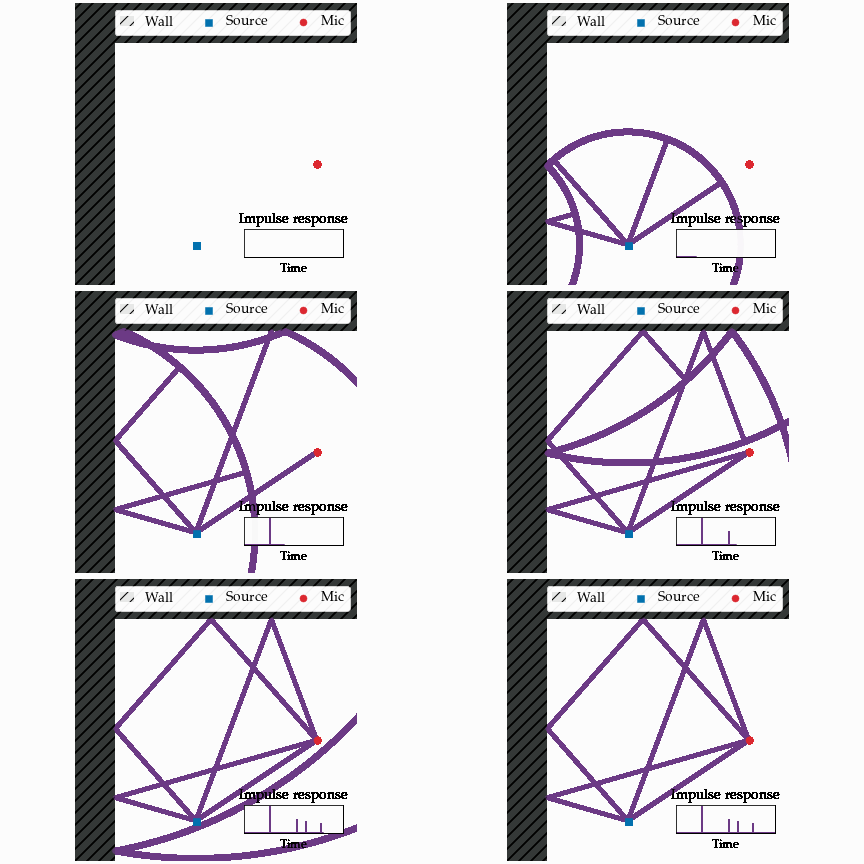
Fig. 54 A room’s impulse response builds up from the direct sound plus a growing collection of delayed, attenuated reflections off the walls. Convolving a dry signal with this response simulates playing the signal in the room. Animation is borrowed with permission from Digital Signals Theory [McF23] (source).

With a recorded impulse response in hand, applying convolution reverb is just a single convolution. The example below convolves a dry marimba loop with the recorded impulse response of a real church (resampling the dry sound to match the impulse response’s sample rate first). Listen for the way the marimba suddenly acquires the long, echoing tail of the space:

# hide
import numpy as np
import pyquist as pq

# Convolution reverb: convolve a dry recording with a room's impulse response
# to make it sound as if it were played in that room.
dry = pq.Audio.from_file("./assets/audio-reverb-dry.wav")
ir = pq.Audio.from_file("./assets/audio-reverb-ir.wav")

print("Dry marimba loop:")
pq.play(dry, normalize=True)
print("Room impulse response (the recorded reverb tail):")
pq.play(ir, normalize=True)

dry = dry.resample(ir.sample_rate)                # match sample rates first
x = np.asarray(dry.samples).reshape(-1)
h = np.asarray(ir.samples).reshape(-1)

wet = np.convolve(x, h)                            # apply the room

print("Wet signal (the marimba convolved with the room):")
pq.play(pq.Audio(wet, ir.sample_rate), normalize=True)

Dry marimba loop:

Room impulse response (the recorded reverb tail):

Wet signal (the marimba convolved with the room):

Note

Dry sound: Marimba loop 3 by BrickDeveloper171, License: CC0. Impulse response: IR_Church_01 by snapssound, License: Attribution 4.0.