1.1 Waveforms: sound as a continuous function

Formally, we describe an analog sound by a function

\[p(t) : \mathbb{R} \to \mathbb{R},\]

mapping a real-valued time \(t\) (seconds) to a real-valued pressure \(p(t)\). We refer to such a function as a waveform, or more generally as a (continuous-time) signal.

Why [-1, 1]?

Normalizing to a unitless range is hardware-agnostic — the same code works across different bit depths, file formats, and audio systems.

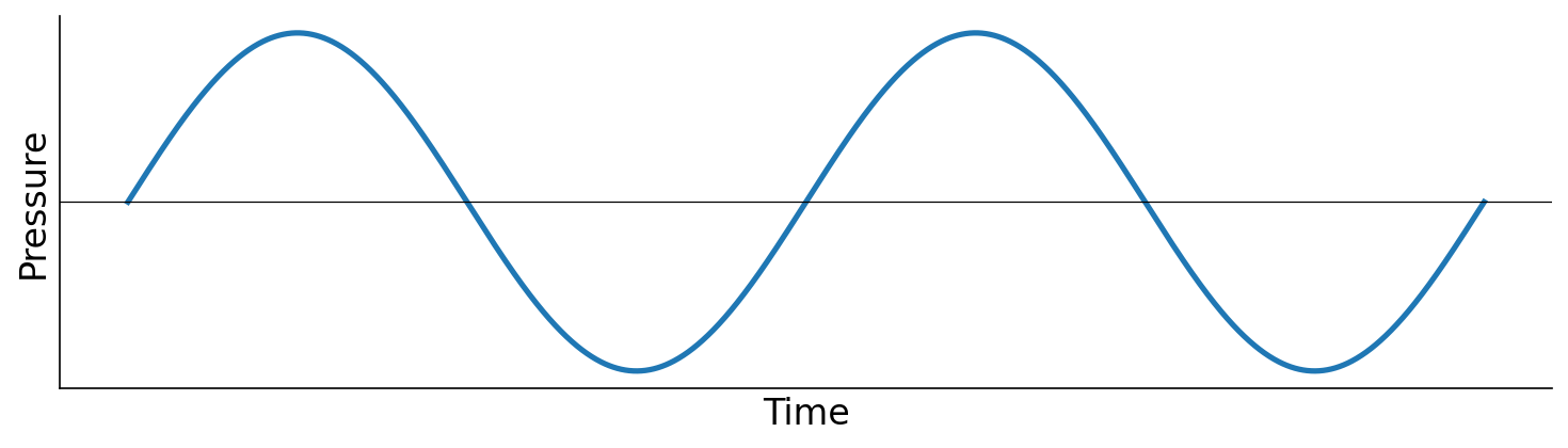
To represent natural sound, \(p(t)\) characterizes the air pressure at a fixed point in space over time. Pressure can be measured in physical units like Pascals, but in computer music we usually work with a unitless, normalized representation. Once a sound is recorded through a microphone (or otherwise scaled to a known range), we refer to the measured quantity as amplitude, and we linearly rescale it so that the recording system’s full dynamic range maps to the interval \([-1, 1]\):

\[x(t) : \mathbb{R} \to [-1, 1]\]

A key aspect of this rescaling is that amplitude is proportional to pressure. Concretely, \(x(t) = p(t) / p_{\max}\), where \(p(t)\) is the underlying pressure signal (e.g., in Pascals) and \(p_{\max} = \max_{t \in \mathbb{R}} |p(t)|\) is the maximum pressure magnitude the recording system can represent. Unless otherwise specified, you should henceforth imagine the vertical axis of a waveform plot as a unitless amplitude in \([-1, 1]\): \(+1\) is the maximum positive deviation the system can represent, \(-1\) is the maximum negative deviation, and \(0\) is silence.