import matplotlib
if not hasattr(matplotlib.RcParams, "_get"):
    matplotlib.RcParams._get = dict.get

8.7 Analyzing and reconstructing a real sound

Let us put the DFT to work on a real recording: a single clarinet note. Analysis and resynthesis together demonstrate the round trip between time and frequency that this chapter has built toward. Here is the note we will be working with:

The clarinet recording we will analyze and then resynthesize from its spectrum. 356930 by MTG, License: Attribution 3.0.

Analysis

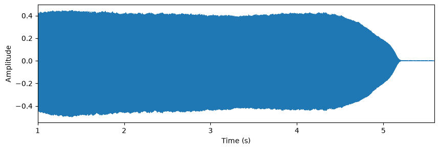
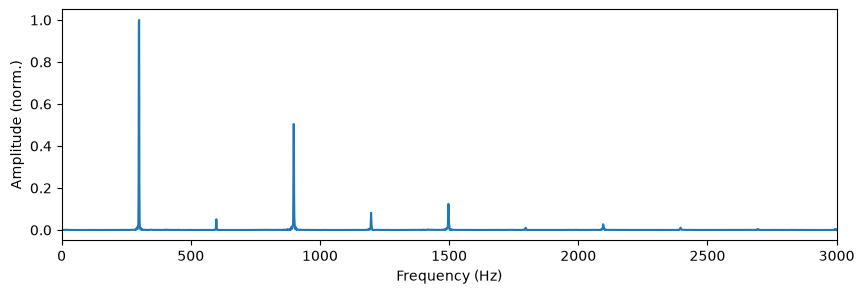
First we analyze the sound, viewing it in both domains. In the time domain, we plot the waveform from just before the note begins through to the end, which reveals its overall envelope: a fast “attack”, a long “sustain”, and a slow “release”. In the frequency domain, we take the DFT (via np.fft.rfft) of a stable segment and plot the amplitude spectrum:

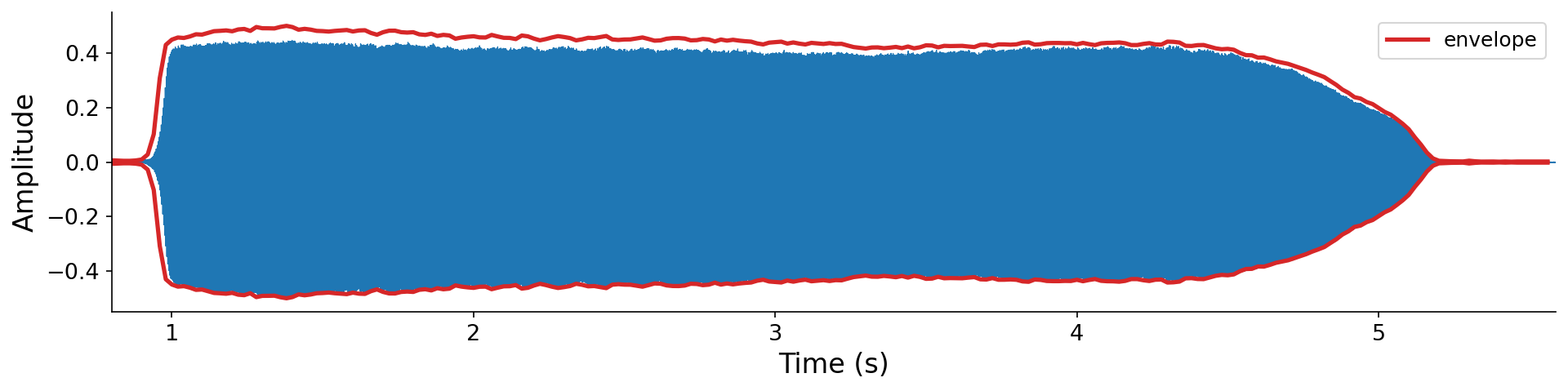
Fig. 46 The clarinet note in the time domain, starting just before its onset. At this zoom the individual oscillations blur together into a solid band, but the smooth red curve tracing the waveform’s peaks shows the envelope clearly: a quick attack rising to a peak near 1.4 s, a long sustain, and a gradual release.

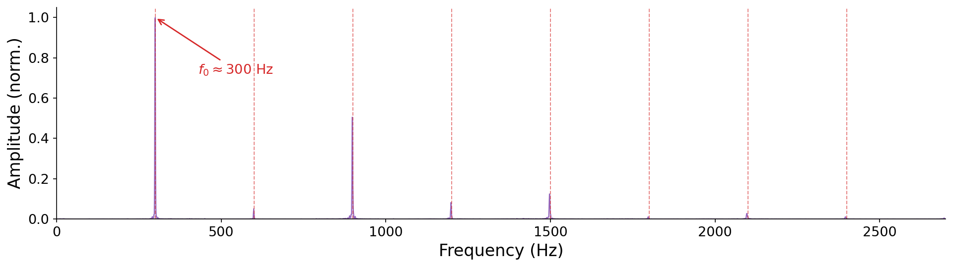
Fig. 47 The clarinet’s amplitude spectrum from the DFT. The fundamental sits at \(f_0 \approx 300\) Hz, and the note is dominated by its odd harmonics (3rd at 900 Hz, 5th at 1500 Hz), with the even harmonics strongly suppressed. This odd-harmonic signature is characteristic of the clarinet. We will understand why when we examine instrument acoustics later on.

From these two plots we can read off, by eye, a recipe for the sound: its fundamental frequency (\(f_0 \approx 300\) Hz), the amplitudes of its harmonics (strong odds, weak evens, taken from the spectral peaks), and the shape of its envelope (from the time-domain outline). The interactive example below performs this analysis in code:

# hide
import numpy as np
import matplotlib.pyplot as plt
import pyquist as pq

# Load the clarinet note and plot its waveform from 1 second onward.
clarinet = pq.Audio.from_file("./assets/audio-clarinet.wav")
x = np.asarray(clarinet.samples).reshape(-1)
sr = clarinet.sample_rate

t = np.arange(len(x)) / sr
plt.figure(figsize=(10, 3))
plt.plot(t, x, linewidth=0.5)
plt.xlim(1.0, len(x) / sr)
plt.xlabel("Time (s)"); plt.ylabel("Amplitude")
plt.show()

# Amplitude spectrum of a stable one-second segment, via the real FFT.
seg = x[int(1.0 * sr):int(2.0 * sr)] * np.hanning(sr)
X = np.abs(np.fft.rfft(seg))
freqs = np.fft.rfftfreq(len(seg), 1 / sr)

plt.figure(figsize=(10, 3))
plt.plot(freqs, X / X.max())
plt.xlim(0, 3000)
plt.xlabel("Frequency (Hz)"); plt.ylabel("Amplitude (norm.)")
plt.show()

# pyquist also provides pq.plot_freq, a built-in shortcut for inspecting audio
# in the frequency domain (it computes and plots the amplitude spectrum for you):
# pq.plot_freq(clarinet)

Resynthesis

Now we run the process backwards. Using the fundamental, harmonic amplitudes, and envelope we just extracted, we can resynthesize the note with the additive synthesis of Chapter 3, summing harmonics and applying the envelope:

Original clarinet

Resynthesized from its spectrum

The original recording (above) alongside an additive resynthesis built only from the fundamental, harmonic amplitudes, and envelope read off the DFT analysis. It is not a perfect copy (we discarded the phases, the exact harmonic evolution, and the breathy attack transient), but the pitch and characteristic timbre come through.

The interactive example below hardcodes the extracted parameters and produces the playable resynthesis, so you can experiment with the recipe:

# hide
import numpy as np
import pyquist as pq

F_S = 44100

# The recipe read off the DFT analysis. Edit these values and re-run to hear
# how each ingredient shapes the sound.
f0 = 300.0                                  # fundamental frequency (Hz)
harmonic_amps = [1.00, 0.05, 0.51, 0.08,    # amplitude of each harmonic;
                 0.12, 0.01, 0.03, 0.01]    # the odd harmonics dominate
envelope = [(0.0, 0.0), (0.08, 1.0),        # (time in seconds, level)
            (2.7, 1.0), (3.0, 0.0)]

K, T = len(harmonic_amps), envelope[-1][0]
N = int(T * F_S)
t = (np.arange(N) / F_S)[np.newaxis, :]
k = (np.arange(K) + 1)[:, np.newaxis]
a = np.array(harmonic_amps)[:, np.newaxis]
x_harms = a * np.sin(2 * np.pi * k * f0 * t)
x = x_harms.sum(axis=0)
env = np.interp(t[0], [p[0] for p in envelope], [p[1] for p in envelope])

audio = pq.Audio(x * env, F_S).normalize()
pq.play(audio)

Hopefully you agree from this example that the DFT is a powerful technique! We can synthesize a recognizable clarinet sound just by reading a handful of numbers straight off of the amplitude spectrum and combining with a basic amplitude envelope.