import matplotlib
if not hasattr(matplotlib.RcParams, "_get"):
    matplotlib.RcParams._get = dict.get

6.6 FM sidebands

Vibrato is FM with a slow, shallow modulator. But the real power of FM appears when the modulator runs at audio rates. Recall the trumpet from the introduction, whose harmonics shift in balance continuously over time. Reproducing that with additive synthesis would demand many oscillators, each with its own time-varying amplitude. FM offers a wildly more efficient route.

Just as with ring and amplitude modulation, FM produces sidebands. But where those techniques produced only two, FM produces a theoretically infinite series of sidebands, spaced evenly around the carrier at

\[f_c \pm k \cdot f_m, \qquad k \in \mathbb{Z}^+.\]

This is the key to FM’s efficiency. Two oscillators can generate an arbitrarily rich spectrum. The following figure shows the finite (three-line) spectrum of amplitude modulation with the infinite (many-line) spectrum of frequency modulation:

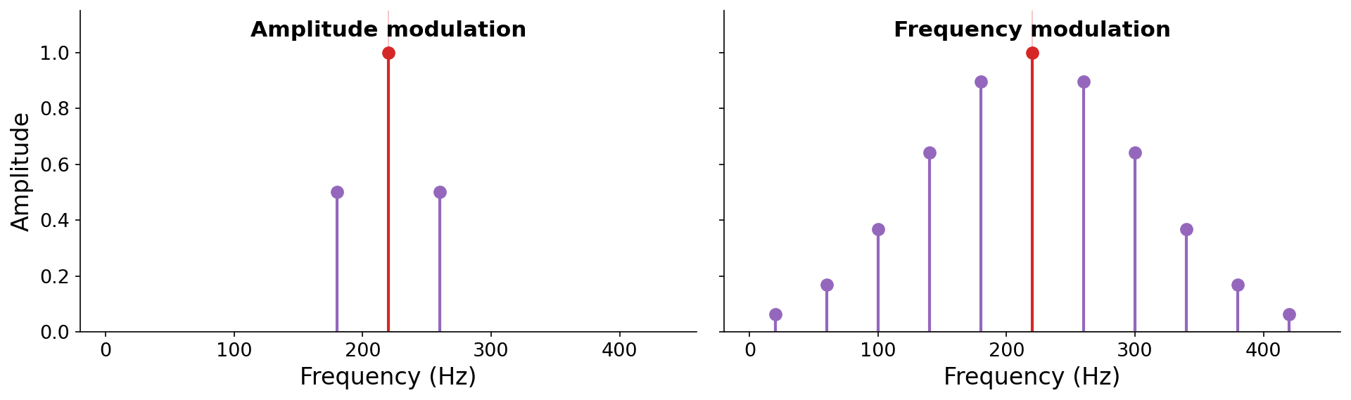
Fig. 29 Amplitude modulation (left) creates just two sidebands, while frequency modulation (right) creates an entire series of sidebands at \(f_c \pm k f_m\). The FM spectrum shown is schematic. The next figure measures the real thing.

Two parameters shape the FM spectrum. First, the ratio \(f_c / f_m\) determines the harmonicity of the result. When \(f_c / f_m\) is a simple rational number, many of the sidebands land on integer multiples of a common fundamental, producing a harmonic, pitched tone. When the ratio is irrational, the sidebands are inharmonic, producing bell-like or metallic timbres.

Harmonic, \(f_c/f_m = 2\)

Inharmonic, \(f_c/f_m = \sqrt{2}\)

Two FM tones at the same index of modulation (\(I = 3\)). Left: a simple ratio (\(f_c = 440\) Hz, \(f_m = 220\) Hz) lands the sidebands on integer multiples of a common fundamental, giving a harmonic, pitched tone. Right: the irrational ratio \(f_c/f_m = \sqrt{2}\) (\(f_c = 440\) Hz, \(f_m = 440/\sqrt{2} \approx 311\) Hz) gives an inharmonic, bell-like timbre.

Second, the number of audible sidebands is controlled by the index of modulation, the unitless ratio of the depth of modulation (\(D\), in Hz) to the rate of modulation (\(f_m\), also in Hz):

\[I = \frac{D}{f_m}.\]

As \(I\) grows, energy spreads from the carrier out into more and more sidebands, and the tone brightens. A useful rule of thumb is that roughly \(I + 1\) sidebands are audible on each side of the carrier. The following figure measures the actual FM spectrum (via the Fourier transform) as the index of modulation increases:

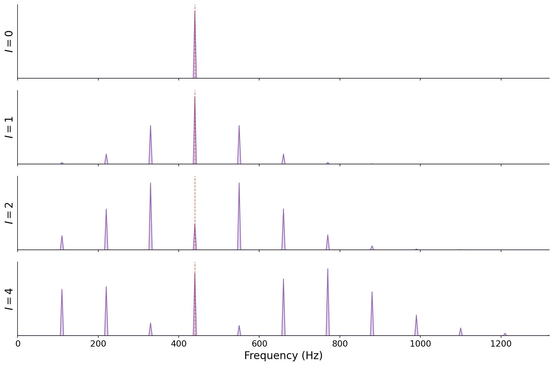
Fig. 30 The measured spectrum of an FM tone (\(f_c = 440\) Hz, \(f_m = 110\) Hz) as the index of modulation \(I\) increases. At \(I = 0\) there is only the carrier. As \(I\) grows, sidebands appear at \(f_c + k f_m\) and energy spreads outward, roughly \(I + 1\) sidebands to a side.

Index of modulation 1

Index of modulation 2

Index of modulation 4

The same carrier and modulator (\(f_c = 440\) Hz, \(f_m = 110\) Hz) at increasing index of modulation. The tone grows brighter and richer as more sidebands become audible.

The exact amplitudes of the FM sidebands are given by mathematical functions (Bessel functions) whose derivation is beyond the scope of this book. What matters here is the qualitative picture: by carefully controlling \(f_c\), \(f_m\), and especially the index of modulation \(I\) over the duration of a note, we can emulate sophisticated, evolving instrumental spectra with just two oscillators. This is exactly how the FM synthesizers of the 1980s produced their signature sounds, which were our very first source of inspiration back in Chapter 0.

Explore how the parameters shape the spectrum for yourself. The widget below plots the FM waveform and its sidebands as you vary the carrier frequency, modulating frequency, and index of modulation:

# hide
# no-output
from IPython.utils.capture import capture_output
with capture_output():
    %pip install -q plotly anywidget

import asyncio
import os
import numpy as np
import plotly.graph_objects as go
from plotly.subplots import make_subplots
import ipywidgets as widgets
from IPython.display import Audio
import icm_plotly
from icm_plotly import RED, BLUE

Play with the classic FM parameters from the definition above: the carrier frequency \(f_c\), the modulating frequency \(f_m\), and the index of modulation \(I = D/f_m\). The waveform \(\sin(2\pi f_c t + I\sin(2\pi f_m t))\) is on the left, and its spectrum (the carrier and its sidebands at \(f_c \pm k f_m\)) is on the right. The audio card underneath rings the current settings like a bell.

# hide
# autorun
FC0, FM0, I0 = 220.0, 220.0, 2.0        # starting parameters

t_wave = np.linspace(0.0, 0.02, 1200)   # 20 ms of waveform
N = 4096                                # spectrum: ~93 ms, hann-windowed
sr = 44100
t_spec = np.arange(N) / sr
win = np.hanning(N)
freqs = np.fft.rfftfreq(N, 1 / sr)
mask = freqs <= 5000
t_bell = np.arange(2 * sr) / sr          # two seconds, for the ear
env = np.exp(-3 * t_bell)               # a bell's decay

def fm(fc, fm_, I, t):
    return np.sin(2 * np.pi * fc * t + I * np.sin(2 * np.pi * fm_ * t))

def spectrum(fc, fm_, I):
    X = np.abs(np.fft.rfft(fm(fc, fm_, I, t_spec) * win))
    return X[mask] / X.max()

def figure():
    fig = make_subplots(rows=1, cols=2, horizontal_spacing=0.12)
    fig.add_scatter(x=t_wave * 1000, y=fm(FC0, FM0, I0, t_wave),
                    mode="lines", line=dict(color=RED, width=1.8),
                    row=1, col=1)
    fig.add_scatter(x=freqs[mask], y=spectrum(FC0, FM0, I0),
                    mode="lines", line=dict(color=BLUE, width=1.5),
                    row=1, col=2)
    fig.update_xaxes(range=[0, 20], title_text="Time (ms)",
                     fixedrange=True, row=1, col=1)
    fig.update_yaxes(range=[-1.1, 1.1], title_text="Amplitude",
                     fixedrange=True, row=1, col=1)
    fig.update_xaxes(range=[0, 5000], title_text="Frequency (Hz)",
                     fixedrange=True, row=1, col=2)
    fig.update_yaxes(range=[0, 1.05], title_text="Magnitude",
                     fixedrange=True, row=1, col=2)
    return fig

def controls(fig):
    fc = widgets.FloatSlider(description="Carrier f_c (Hz)", min=55, max=880,
                             value=FC0, step=5)
    fmod = widgets.FloatSlider(description="Modulator f_m (Hz)", min=55,
                               max=880, value=FM0, step=5)
    idx = widgets.FloatSlider(description="Index I", min=0, max=10, value=I0,
                              step=0.1)

    # the defaults snapshot the arrays; the page's notebooks share one kernel
    def update(fc, fm_, I, t_wave=t_wave, fm=fm, spectrum=spectrum):
        with fig.batch_update():
            fig.data[0].y = fm(fc, fm_, I, t_wave)
            fig.data[1].y = spectrum(fc, fm_, I)

    widgets.interactive_output(update, {"fc": fc, "fm_": fmod, "I": idx})

    # the audio card under the controls: the previous clip stays in place
    # while you drag (so the layout never jumps) and is swapped for the new
    # one when the pointer releases (keyboard nudges settle on a timer). It is
    # written through the Output's synced `outputs` trait, which works
    # outside a kernel message, where display() output has no destination
    out = widgets.Output()
    gate = icm_plotly.release_gate()   # pointer state: is a slider mid-drag?
    pending = []
    dirty = []

    def render(t=t_bell, env=env, sr=sr):
        # a bell: index and amplitude decay together, which makes it ring
        x = env * np.sin(2 * np.pi * fc.value * t
                         + idx.value * env * np.sin(2 * np.pi * fmod.value * t))
        x *= 0.125 / np.abs(x).max()          # about -18 dBFS, a safe level
        audio = Audio(x.astype(np.float32), rate=sr, normalize=False)
        data, metadata = get_ipython().display_formatter.format(audio)
        # one assignment swaps the old card for the new one in place, so
        # the page never shows an empty card and nothing shifts
        out.outputs = ({"output_type": "display_data",
                        "data": data, "metadata": metadata},)

    async def settle():
        await asyncio.sleep(0.25)
        pending.clear()
        if dirty and not gate.dragging:
            dirty.clear()
            render()

    def on_change(_):
        dirty.append(True)
        if pending:
            pending.pop().cancel()
        pending.append(asyncio.ensure_future(settle()))

    def on_release(change):
        if not change["new"] and dirty:
            if pending:
                pending.pop().cancel()
            dirty.clear()
            render()

    gate.observe(on_release, names="dragging")

    for s in (fc, fmod, idx):
        s.observe(on_change, names="value")
    if not os.environ.get("ICM_BOOK_BUILD"):   # the build bakes no card
        render()
    return widgets.VBox([fc, fmod, idx, out, gate])

icm_plotly.show(figure, controls)

Carrier f_c (Hz)220.00

Modulator f_m (Hz)220.00

Index I2.00