6.3 Amplitude modulation

import matplotlib
if not hasattr(matplotlib.RcParams, "_get"):
    matplotlib.RcParams._get = dict.get

6.3 Amplitude modulation#

Our original goal with ring modulation was simply to add a tremolo envelope. But in doing so, we accidentally removed the carrier itself from the spectrum, replacing it with two sidebands. What if we want the tremolo effect while keeping the original carrier tone?

The fix is intuitive: just add the carrier back in. Starting from ring modulation and adding an unmodulated copy of the carrier gives \(\sin(\omega_c t) + \sin(\omega_c t)\,\sin(\omega_m t)\), which we can factor into a cleaner form that also conveniently reduces the number of sinusoids needed for computation. This is amplitude modulation.

Definition 18 (Amplitude modulation)

Amplitude modulation (AM) multiplies a carrier by a modulator that oscillates around a nonzero average:

\[\text{AmpMod}(t) = \sin(\omega_c t)\,\big[1 + \sin(\omega_m t)\big].\]

Expanding the product shows what AM does in the frequency domain. It is just ring modulation plus the original carrier:

\[\sin(\omega_c t)\big[1 + \sin(\omega_m t)\big] = \underbrace{\sin(\omega_c t)}_{\text{carrier}} + \underbrace{\sin(\omega_c t)\sin(\omega_m t)}_{\text{sidebands}}.\]

So the spectrum retains the carrier at \(\omega_c\) with amplitude 1, and adds the two ring-modulation sidebands at \(\omega_c \pm \omega_m\), each with amplitude \(\tfrac{1}{2}\):
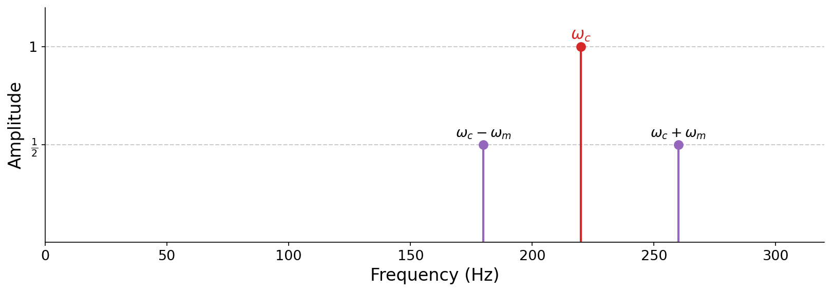
A frequency-domain stem plot with a tall carrier spike at 220 Hz (amplitude 1) flanked by two shorter sidebands at 180 and 260 Hz (amplitude one half each).

Fig. 26 The spectrum of amplitude modulation. Unlike ring modulation, the carrier at \(\omega_c\) survives (amplitude 1), flanked by the two sidebands at \(\omega_c \pm \omega_m\) (amplitude \(\tfrac{1}{2}\)).#

Amplitude modulation. Because the modulator is in the audible range, we hear the carrier at 220 Hz together with its two sidebands, rather than a tremolo.

We can control the balance between the carrier and its sidebands with a ratio parameter \(r\):

\[\text{AmpMod}(t) = \sin(\omega_c t)\,\Big[\tfrac{r}{2} + \sin(\omega_m t)\Big],\]

where \(r\) is the ratio of the carrier’s amplitude to each sideband’s amplitude. Setting \(r = 2\) recovers the definition above where the amplitude of \(\omega_c\) is twice that of the sidebands. Observe that, by carefully configuring \(\omega_c\), \(\omega_m\), and \(r\), amplitude modulation can even be used to design specific harmonic spectra (where all frequency content are integer multiples of a fundamental), an idea we will develop in the exercises at the end of the chapter.

Experiment with amplitude modulation below. Vary the carrier frequency, modulating frequency, and ratio \(r\), then listen and watch how the carrier and its two sidebands move:

# hide
# no-output
from IPython.utils.capture import capture_output
with capture_output():
    %pip install -q plotly anywidget

import asyncio
import os
import numpy as np
import plotly.graph_objects as go
from plotly.subplots import make_subplots
import ipywidgets as widgets
from IPython.display import Audio
import icm_plotly
from icm_plotly import RED, BLUE

Play with the amplitude-modulation parameters: the carrier frequency \(f_c\), the modulating frequency \(f_m\), and the ratio \(r\) of the carrier’s amplitude to each sideband’s amplitude. The waveform \(\sin(2\pi f_c t)\,[\tfrac{r}{2} + \sin(2\pi f_m t)]\) is on the left, and its spectrum (the carrier at \(f_c\) and two sidebands at \(f_c \pm f_m\)) is on the right. The audio card underneath plays the current settings.

# hide
# autorun
FC0, FM0, R0 = 220.0, 55.0, 2.0         # starting parameters

t_wave = np.linspace(0.0, 0.04, 1200)   # 40 ms of waveform
N = 4096                                # spectrum: ~93 ms, hann-windowed
sr = 44100
t_spec = np.arange(N) / sr
win = np.hanning(N)
freqs = np.fft.rfftfreq(N, 1 / sr)
mask = freqs <= 3000
t_play = np.arange(2 * sr) / sr          # two seconds, for the ear

def am(fc, fm_, r, t):
    return np.sin(2 * np.pi * fc * t) * (r / 2 + np.sin(2 * np.pi * fm_ * t))

def spectrum(fc, fm_, r):
    X = np.abs(np.fft.rfft(am(fc, fm_, r, t_spec) * win))
    return X[mask] / X.max()

def figure():
    fig = make_subplots(rows=1, cols=2, horizontal_spacing=0.12)
    fig.add_scatter(x=t_wave * 1000, y=am(FC0, FM0, R0, t_wave),
                    mode="lines", line=dict(color=RED, width=1.8),
                    row=1, col=1)
    fig.add_scatter(x=freqs[mask], y=spectrum(FC0, FM0, R0),
                    mode="lines", line=dict(color=BLUE, width=1.5),
                    row=1, col=2)
    fig.update_xaxes(range=[0, 40], title_text="Time (ms)",
                     fixedrange=True, row=1, col=1)
    fig.update_yaxes(range=[-2.1, 2.1], title_text="Amplitude",
                     fixedrange=True, row=1, col=1)
    fig.update_xaxes(range=[0, 3000], title_text="Frequency (Hz)",
                     fixedrange=True, row=1, col=2)
    fig.update_yaxes(range=[0, 1.05], title_text="Magnitude",
                     fixedrange=True, row=1, col=2)
    return fig

def controls(fig):
    fc = widgets.FloatSlider(description="Carrier f_c (Hz)", min=55, max=880,
                             value=FC0, step=5)
    fmod = widgets.FloatSlider(description="Modulator f_m (Hz)", min=5,
                               max=880, value=FM0, step=5)
    ratio = widgets.FloatSlider(description="Ratio r", min=0, max=4, value=R0,
                                step=0.1)

    # the defaults snapshot the arrays; the page's notebooks share one kernel
    def update(fc, fm_, r, t_wave=t_wave, am=am, spectrum=spectrum):
        with fig.batch_update():
            fig.data[0].y = am(fc, fm_, r, t_wave)
            fig.data[1].y = spectrum(fc, fm_, r)

    widgets.interactive_output(update, {"fc": fc, "fm_": fmod, "r": ratio})

    # the audio card under the controls: the previous clip stays in place
    # while you drag (so the layout never jumps) and is swapped for the new
    # one when the pointer releases (keyboard nudges settle on a timer). It is
    # written through the Output's synced `outputs` trait, which works
    # outside a kernel message, where display() output has no destination
    out = widgets.Output()
    gate = icm_plotly.release_gate()   # pointer state: is a slider mid-drag?
    pending = []
    dirty = []

    def render(t=t_play, sr=sr):
        x = am(fc.value, fmod.value, ratio.value, t)
        fade = int(0.01 * sr)          # 10 ms fade in/out to avoid clicks
        x[:fade] *= np.linspace(0, 1, fade)
        x[-fade:] *= np.linspace(1, 0, fade)
        x *= 0.2 / np.abs(x).max()     # a safe playback level
        audio = Audio(x.astype(np.float32), rate=sr, normalize=False)
        data, metadata = get_ipython().display_formatter.format(audio)
        # one assignment swaps the old card for the new one in place, so
        # the page never shows an empty card and nothing shifts
        out.outputs = ({"output_type": "display_data",
                        "data": data, "metadata": metadata},)

    async def settle():
        await asyncio.sleep(0.25)
        pending.clear()
        if dirty and not gate.dragging:
            dirty.clear()
            render()

    def on_change(_):
        dirty.append(True)
        if pending:
            pending.pop().cancel()
        pending.append(asyncio.ensure_future(settle()))

    def on_release(change):
        if not change["new"] and dirty:
            if pending:
                pending.pop().cancel()
            dirty.clear()
            render()

    gate.observe(on_release, names="dragging")

    for s in (fc, fmod, ratio):
        s.observe(on_change, names="value")
    if not os.environ.get("ICM_BOOK_BUILD"):   # the build bakes no card
        render()
    return widgets.VBox([fc, fmod, ratio, out, gate])

icm_plotly.show(figure, controls)
Carrier f_c (Hz)220.00
Modulator f_m (Hz)55.00
Ratio r2.00