8.3 Issue 3: Finite frequencies

We have discretized time, but not frequency. The sum from the previous section can be evaluated at any real \(\omega\), but our goal is to discover the frequency content of \(x[n]\). Accordingly, we face a catch-22: how do we know which \(\omega\) values to test if we know nothing about the signal in advance? There are infinitely many to choose from.

Here sampling theory rescues us again. Recall from Chapter 7 that a signal sampled at rate \(f_s\) can only carry frequency content in the range \([-\tfrac{f_s}{2}, \tfrac{f_s}{2}]\). Anything outside that range aliases back into it. That immediately shrinks our search from all of \(\mathbb{R}\) down to a bounded interval of width \(f_s\). But there are still infinitely many real frequencies inside it.

The key idea is to simply pick a finite set of frequencies that evenly covers the range. For \(N\) samples, we choose exactly \(N\) frequencies, spaced uniformly across the bandwidth \(f_s\). Their spacing is therefore

\[\Delta f = \frac{f_s}{N} = \frac{1}{N \Delta t}.\]

Indexing these frequencies by an integer \(k\), the \(k\)-th analysis frequency is the one that completes exactly \(k\) cycles over the \(N \Delta t\) seconds spanned by the window. In cycles per second, that is

\[f_k = \frac{k}{N \Delta t} \quad \left[ \frac{\text{cycles}}{\text{second}} \right], \qquad k \in \{0, 1, \ldots, N-1\},\]

and multiplying by \(2\pi\) \(\frac{\text{radians}}{\text{cycle}}\) converts it to angular frequency,

\[\omega_k = 2\pi f_k = \frac{2\pi k}{N \Delta t} \quad \left[ \frac{\text{radians}}{\text{second}} \right].\]

Now watch what happens when we form the corresponding analysis phasor \(e^{-j\omega_k n \Delta t}\). The sampling period \(\Delta t\) cancels out completely:

\[e^{-j\omega_k n \Delta t} = e^{-j \frac{2\pi k}{N \Delta t}\, n \Delta t} = e^{-2\pi j k n / N}.\]

This is a key observation: the analysis phasor no longer depends on the sampling rate at all. It depends only on the bin index \(k\), the sample index \(n\), and the total number of samples \(N\). The following figure plots the real (\(\cos\)) and imaginary (\(-\sin\)) parts of these phasors for the first few \(k\):

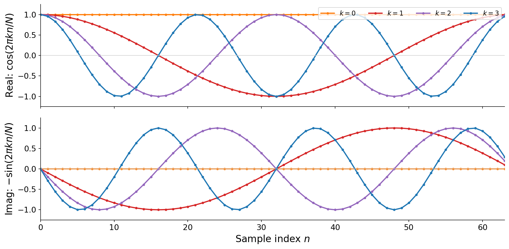
Fig. 44 The analysis phasors \(e^{-j\omega_k n\Delta t} = e^{-2\pi j k n / N}\) for \(k = 0, 1, 2, 3\) (here \(N = 64\)), split into their real (\(\cos\)) and imaginary (\(-\sin\)) parts. Higher \(k\) means a higher-frequency phasor, completing \(k\) cycles across the window. This is reminiscent of the harmonics of additive synthesis from Chapter 3.

Note

Why index \(k\) from \(0\) to \(N-1\), covering \([0, f_s)\), rather than the symmetric range \([-\tfrac{f_s}{2}, \tfrac{f_s}{2}]\) we might expect? The two are equivalent because of aliasing. A bin \(k\) in the upper half, with frequency \(f_k = k f_s / N\) above the Nyquist frequency \(f_s/2\), is an exact alias of the negative frequency \(f_k - f_s\). So the second half of the bins, \(k = \tfrac{N}{2}+1, \ldots, N-1\), simply represents the negative frequencies \(-\tfrac{f_s}{2}, \ldots, 0\). Convention indexes them as \(0\) to \(N-1\) because that is how they fall out of the math, but you should interpret the upper half as the negative frequencies folded around.