import matplotlib
if not hasattr(matplotlib.RcParams, "_get"):
    matplotlib.RcParams._get = dict.get

7.2 Aliasing

What happens when we sample too slowly? Return to the sinusoids that shared identical samples, now adding a third at 4 Hz. Sampled at \(f_s = 1\) Hz, all three still land on their zero crossings, so they remain indistinguishable:

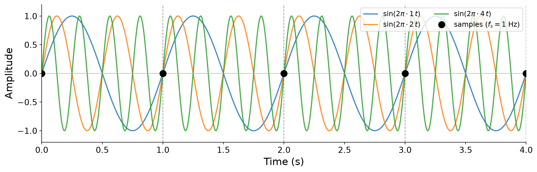
Fig. 37 The same picture with a third sinusoid at 4 Hz. At \(f_s = 1\) Hz, the 1, 2, and 4 Hz tones share identical (all-zero) samples, so from the samples alone we cannot tell them apart.

From the samples alone, a 1 Hz signal and a 4 Hz signal are indistinguishable. When we undersample, high frequencies masquerade as lower ones. This phenomenon is called aliasing, and the impostor frequencies are called aliases.

When sampling by \(f_s\), every frequency has infinitely many aliases, spaced \(f_s\) apart. For a frequency \(f\), its aliases are the set

\[\text{Alias}_f = \{\, f + k \cdot f_s \mid k \in \mathbb{Z} \,\},\]

all the frequencies that differ from \(f\) by an integer multiple of the sampling rate. This is exactly the copied-spectrum picture: each true frequency shows up again at every multiple of \(f_s\). These aliases are not merely hard to tell apart, they are mathematically identical: a tone at \(f\) and a tone at any of its aliases produce the exact same samples. So when the samples are reconstructed, the signal necessarily comes back at the single alias that falls within the Nyquist band \([0, f_s/2]\). We can compute that apparent frequency directly:

Definition 21 (Aliased frequency)

When a frequency \(f\) is sampled at rate \(f_s\), its apparent (aliased) frequency is

\[f_{\text{alias}} = \min\big(f \bmod f_s,\; f_s - (f \bmod f_s)\big),\]

which always lies in \([0, f_s/2]\). If \(f\) is already in \([0, f_s/2]\), then \(f_{\text{alias}} = f\) and no aliasing occurs. Otherwise \(f_{\text{alias}} \neq f\).

Aliasing in practice

Aliasing is a very real, audible phenomenon, not just a theoretical construct. To hear it, we can synthesize a tone whose frequency slowly sweeps up from 220 Hz to 880 Hz and back, at a few different sample rates. The following clips were each synthesized directly at the given \(f_s\) (then resampled purely for playback), so any aliasing is baked into the sound:

Sweep at f_s = 2000 Hz

Sweep at f_s = 1000 Hz

Sweep at f_s = 500 Hz

The same 220-to-880 Hz frequency sweep synthesized at three sample rates. At \(f_s = 2000\) Hz the sweep is clean. As \(f_s\) drops, the upper part of the sweep exceeds the Nyquist frequency and folds back down, so the perceived frequency audibly reverses direction.

The figure below plots what is happening. The true frequency (blue) rises above the Nyquist frequency (red) once \(f_s\) is small enough, and the frequency we actually hear (orange) folds back below it:

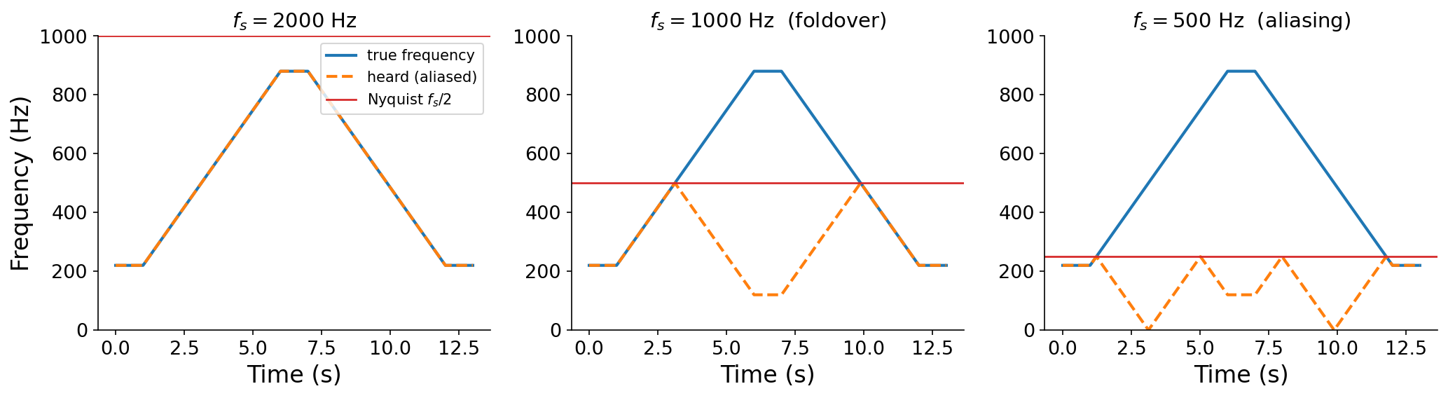
Fig. 38 The frequency sweep at three sample rates. When the true frequency (blue) crosses the Nyquist frequency \(f_s/2\) (red), the heard frequency (orange) reflects back downward. The full sonification code is available as an interactive example below.

For frequencies just above the Nyquist frequency, in the range \([f_s/2, f_s]\), this reflection is colloquially called foldover, because the aliased frequencies mirror back across the Nyquist frequency as if it were a crease in a folded sheet of paper.

The widget below samples a single tone at a rate of your choosing. The true tone and its alias pass through exactly the same samples, which is why nothing downstream can tell them apart.

# hide
# no-output
from IPython.utils.capture import capture_output
with capture_output():
    %pip install -q plotly anywidget

import asyncio
import os
import numpy as np
import plotly.graph_objects as go
from plotly.subplots import make_subplots
import ipywidgets as widgets
from IPython.display import Audio
import icm_plotly
from icm_plotly import RED, BLUE, GOLD, IRON, TEAL, STEEL

Drag the two sliders. On the left, the gray curve is the true tone, the red dots are the samples taken at \(f_s\), and the gold curve is the alias that runs through the very same dots. On the right, the gold line maps every true frequency to the one you actually hear. The audio card plays the current setting.

# hide
# autorun
F0, FS0 = 300.0, 1400.0             # starting parameters

T_WIN = 0.006                       # six milliseconds on screen
t = np.linspace(0.0, T_WIN, 1200)
SR = 44100                          # playback rate
T_PLAY = np.arange(int(1.2 * SR)) / SR
FGRID = np.linspace(0.0, 1250.0, 700)

def alias(f, fs):
    # the chapter's formula, plus the sign the reconstruction comes back with
    m = np.mod(f, fs)
    return min(m, fs - m), (1.0 if m <= fs / 2 else -1.0)

def fold(fs, grid=FGRID):
    m = np.mod(grid, fs)
    return np.minimum(m, fs - m)

def samples(f, fs):
    n = np.arange(int(np.ceil(T_WIN * fs)) + 1)
    return n / fs, np.sin(2 * np.pi * f * n / fs)

def figure():
    fig = make_subplots(rows=1, cols=2, horizontal_spacing=0.13)
    fa, sign = alias(F0, FS0)
    xs, ys = samples(F0, FS0)
    fig.add_scatter(x=t * 1000, y=np.sin(2 * np.pi * F0 * t), mode="lines",
                    line=dict(color=STEEL, width=1.6), row=1, col=1)
    fig.add_scatter(x=t * 1000, y=sign * np.sin(2 * np.pi * fa * t),
                    mode="lines", line=dict(color=GOLD, width=2.2),
                    row=1, col=1)
    fig.add_scatter(x=xs * 1000, y=ys, mode="markers",
                    marker=dict(color=RED, size=7), row=1, col=1)
    fig.add_scatter(x=[0, 1250], y=[0, 1250], mode="lines",
                    line=dict(color=STEEL, width=1.2, dash="dot"),
                    row=1, col=2)
    fig.add_scatter(x=FGRID, y=fold(FS0), mode="lines",
                    line=dict(color=GOLD, width=2.2), row=1, col=2)
    fig.add_scatter(x=[F0], y=[fa], mode="markers",
                    marker=dict(color=RED, size=12,
                                line=dict(color="white", width=2)),
                    row=1, col=2)
    fig.update_xaxes(range=[0, T_WIN * 1000], title_text="Time (ms)",
                     fixedrange=True, row=1, col=1)
    fig.update_yaxes(range=[-1.15, 1.15], title_text="Amplitude",
                     fixedrange=True, row=1, col=1)
    fig.update_xaxes(range=[0, 1250], title_text="True frequency (Hz)",
                     fixedrange=True, row=1, col=2)
    fig.update_yaxes(range=[0, 1250], title_text="Heard frequency (Hz)",
                     fixedrange=True, row=1, col=2)
    return fig

def controls(fig):
    f = widgets.FloatSlider(description="Tone $f$ (Hz)", min=50, max=1200,
                            value=F0, step=10)
    fs = widgets.FloatSlider(description="Sample rate $f_s$ (Hz)", min=400,
                             max=2400, value=FS0, step=50)
    readout = widgets.HTML()

    # the defaults snapshot the arrays; the page's notebooks share one kernel
    def update(f, fs, t=t, alias=alias, fold=fold, samples=samples,
               readout=readout):
        fa, sign = alias(f, fs)
        xs, ys = samples(f, fs)
        with fig.batch_update():
            fig.data[0].y = np.sin(2 * np.pi * f * t)
            fig.data[1].y = sign * np.sin(2 * np.pi * fa * t)
            fig.data[2].x, fig.data[2].y = xs * 1000, ys
            fig.data[4].y = fold(fs)
            fig.data[5].x, fig.data[5].y = [f], [fa]
        note = ("no aliasing" if abs(fa - f) < 1e-9
                else f"heard as <i>f</i><sub>alias</sub> = {fa:.0f} Hz")
        readout.value = (f"<span style='font-size:0.9em'><i>f</i><sub>s</sub>/2 = "
                         f"{fs / 2:.0f} Hz &nbsp;·&nbsp; {note}</span>")

    widgets.interactive_output(update, {"f": f, "fs": fs})

    # the audio card under the controls: the previous clip stays in place
    # while you drag (so the layout never jumps) and is swapped for the new
    # one when the pointer releases (keyboard nudges settle on a timer). It is
    # written through the Output's synced `outputs` trait, which works
    # outside a kernel message, where display() output has no destination
    out = widgets.Output()
    gate = icm_plotly.release_gate()   # pointer state: is a slider mid-drag?
    pending = []
    dirty = []

    def render(T_PLAY=T_PLAY, SR=SR, alias=alias):
        fa, sign = alias(f.value, fs.value)
        # reconstructing those samples gives back exactly one sinusoid, the
        # alias, so we synthesize it directly at the playback rate
        x = sign * 0.125 * np.sin(2 * np.pi * fa * T_PLAY)   # about -18 dBFS
        x[:441] *= np.linspace(0, 1, 441)
        x[-441:] *= np.linspace(1, 0, 441)
        audio = Audio(x.astype(np.float32), rate=SR, normalize=False)
        data, metadata = get_ipython().display_formatter.format(audio)
        # one assignment swaps the old card for the new one in place, so
        # the page never shows an empty card and nothing shifts
        out.outputs = ({"output_type": "display_data",
                        "data": data, "metadata": metadata},)


    async def settle():
        await asyncio.sleep(0.25)
        pending.clear()
        if dirty and not gate.dragging:
            dirty.clear()
            render()

    def on_change(_):
        dirty.append(True)
        if pending:
            pending.pop().cancel()
        pending.append(asyncio.ensure_future(settle()))

    def on_release(change):
        if not change["new"] and dirty:
            if pending:
                pending.pop().cancel()
            dirty.clear()
            render()

    gate.observe(on_release, names="dragging")

    for s in (f, fs):
        s.observe(on_change, names="value")
    if not os.environ.get("ICM_BOOK_BUILD"):   # the build bakes no card
        render()
    return widgets.VBox([f, fs, readout, out, gate])

icm_plotly.show(figure, controls)

Tone \(f\) (Hz)300.00

Sample rate \(f_s\) (Hz)1400.00

f_s/2 = 700 Hz  ·  no aliasing

You can explore this yourself. The interactive example below lets you set the sample rate and the frequency contour, then synthesizes and plays the result so you can hear aliasing emerge as you lower \(f_s\):

# hide
import numpy as np
import matplotlib.pyplot as plt
import pyquist as pq

PLAYBACK_SR = 44100


def aliased(f, f_s):
    m = np.mod(f, f_s)
    return np.minimum(m, f_s - m)


def show_aliasing(f_s, control_points):
    # control_points: list of (time_seconds, frequency_hz), interpolated
    # linearly in frequency.
    times = [p[0] for p in control_points]
    freqs = [p[1] for p in control_points]
    dur = times[-1]

    n = np.arange(int(dur * f_s))
    freq = np.interp(n / f_s, times, freqs)

    # synthesize at f_s by accumulating phase (Chapter 6), resample for playback
    x = np.sin(np.cumsum(2 * np.pi * freq / f_s))
    audio = pq.Audio(x.astype(np.float32), int(f_s)).resample(PLAYBACK_SR)

    t = n / f_s
    fig, ax = plt.subplots(figsize=(9, 3.2))
    ax.plot(t, freq, color="#007BC0", label="true frequency")
    ax.plot(t, aliased(freq, f_s), color="#FDB515", ls="--", label="heard (aliased)")
    ax.axhline(f_s / 2, color="#C41230", lw=1.3, label="Nyquist $f_s/2$")
    ax.set_xlabel("Time (s)")
    ax.set_ylabel("Frequency (Hz)")
    ax.set_ylim(0, max(freq.max(), f_s / 2) * 1.15)
    ax.legend(loc="upper right", fontsize=9)
    plt.show()
    return pq.play(audio)

# Edit the sample rate and the frequency contour, then run to see and hear aliasing.
# Each control point is (time in seconds, frequency in Hz).
f_s = 500  # sampling rate (Hz): lower it to force aliasing

freq_contour = [
    (0.0, 220.0),
    (1.0, 220.0),
    (6.0, 880.0),
    (7.0, 880.0),
    (12.0, 220.0),
    (13.0, 220.0),
]

show_aliasing(f_s, freq_contour)

Aliasing beyond audio

Aliasing is not unique to digital audio. It arises whenever any signal is sampled too slowly, including the sampling of light that our eyes and cameras perform. A classic example is the wagon-wheel effect, in which the spoked wheels of a moving vehicle appear to slow down, stop, or even spin backwards on film. A camera captures frames at a fixed rate (its sampling rate). When a wheel rotates by nearly a full spoke-spacing between frames, its true rotation aliases to a much slower apparent rotation, and when it rotates by slightly more than a spoke-spacing, the alias runs backwards (a negative frequency):

You may have experienced the same effect at a concert with a strobe light. The strobe flashes at a fixed rate, sampling the motion of the dancers, and this can make movements appear frozen, slowed, or reversed. The figure below shows a dancer bobbing up and down once per second (a 1 Hz motion). The leftmost panel is the continuous motion, and the other four “sample” it by holding whichever frame was most recently caught by a strobe at the labeled rate, while a shared clock advances:

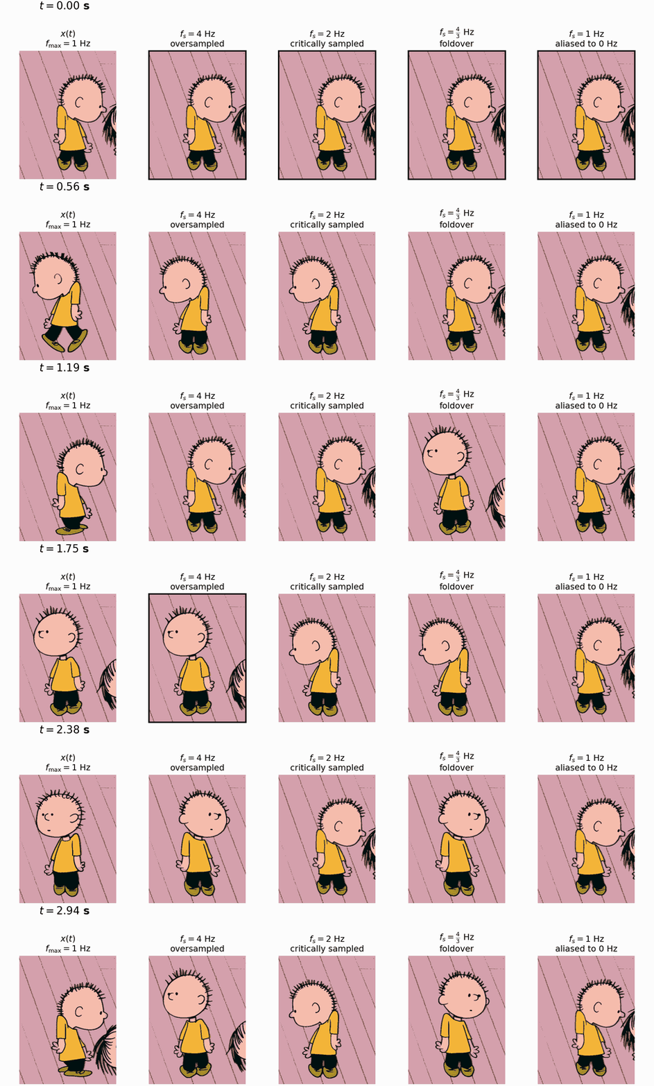
Fig. 39 The same 1 Hz dance, continuous (left) and sampled at four rates. At \(f_s = 4\) Hz the motion still looks correct (oversampled). At \(f_s = 2\) Hz it collapses to just two alternating poses (critical sampling). At \(f_s = 1\) Hz the dancer is caught at the same phase every time and appears frozen, aliased all the way to 0 Hz. At \(f_s = \tfrac{4}{3}\) Hz the dancer appears to dance more slowly, the same foldover we saw with sound.

Critical sampling

The sampling theorem demands \(f_s > 2 f_{\max}\), a strict inequality. What happens right at the boundary, when \(f_s = 2 f_{\max}\)? This edge case is called critical sampling, and it turns out to be genuinely ambiguous.

Consider a cosine at exactly the Nyquist frequency, \(x(t) = \cos(2\pi t)\) with \(f_{\max} = 1\) Hz, sampled at \(f_s = 2\) Hz. The samples are

\[x[n] = \cos(\pi n) = [\,1, -1, 1, -1, \ldots\,],\]

a perfectly reasonable representation of a 1 Hz tone. But now consider a sine at the same frequency, \(x(t) = \sin(2\pi t)\), sampled at the same rate. Its samples are

\[x[n] = \sin(\pi n) = [\,0, 0, 0, 0, \ldots\,].\]

Every sample lands exactly on a zero crossing, so the sine vanishes completely. Those all-zero samples could equally well represent silence, a signal at 0 Hz. At critical sampling, then, a component at exactly \(f_s/2\) may or may not survive, depending on its phase. This is precisely why the theorem requires a strict inequality: at the boundary, reconstruction is no longer guaranteed.