import matplotlib
if not hasattr(matplotlib.RcParams, "_get"):
    matplotlib.RcParams._get = dict.get

3.1 The basic sinusoid#

The most elementary periodic function is the basic sinusoid:

\[x(t) = a \sin(2 \pi f t + \phi).\]

It sounds like a “pure tone” — a smooth, featureless hum with no timbral complexity. As we’ll see later in this chapter, the basic sinusoid is a fundamental building block: all periodic sound, no matter how complex, can be expressed as a sum of basic sinusoids.

The basic sinusoid has three parameters: frequency \(f\), amplitude \(a\), and initial phase \(\phi\).
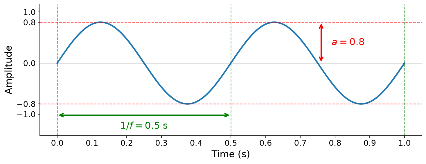
A diagram of the basic sinusoid x(t) = 0.8 sin(2 pi 2 t) with annotations showing amplitude and period

Fig. 3 The sinusoid \(x(t) = 0.8 \sin(2\pi \cdot 2 \, t)\) with \(a = 0.8\), \(f = 2\) Hz, \(\phi = 0\). The dashed red lines mark the amplitude bounds \(\pm a\), and the green dashed lines and arrow mark the period boundaries at \(1/f\).#

Frequency and angular frequency#

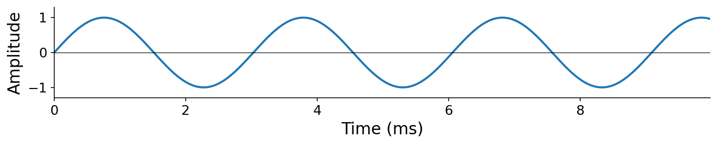
Frequency determines pitch. Listen to pure tones at three different frequencies — each sounds higher in pitch than the last:
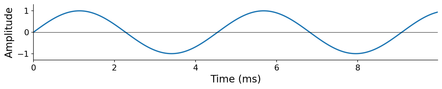
220 Hz sine 220 Hz sine waveform

330 Hz sine 330 Hz sine waveform

440 Hz sine 440 Hz sine waveform

Pure tones at 220, 330, and 440 Hz. Higher frequency means more cycles per second and a higher perceived pitch.

Why does the basic sinusoid with parameter \(f\) complete exactly \(f\) cycles per second? We can reason about this from the units, building up from what we know about \(\sin\).

Recall from trigonometry that \(\sin\) repeats itself with period \(2\pi\) \(\frac{\text{radians}}{\text{cycle}}\). In our basic sinusoid, at \(t = 1\) second, the argument to \(\sin\) will have accumulated \(2\pi f\) radians. This gives us the angular frequency:

\[\omega = 2\pi f \quad \left[\frac{\text{radians}}{\text{second}}\right].\]

To convert back to frequency in Hertz, we divide by \(2\pi\) \(\frac{\text{radians}}{\text{cycle}}\):

\[f = \frac{\omega}{2\pi} \quad \left[\frac{\text{cycles}}{\text{second}}\right].\]

Definition 5 (Angular frequency)

The angular frequency of a sinusoid with frequency \(f\) \(\frac{\text{cycles}}{\text{second}}\) is \(\omega = 2\pi f\) \(\frac{\text{radians}}{\text{second}}\). Equivalently, \(f = \omega / (2\pi)\).

Angular frequency lets us write the basic sinusoid more compactly as \(x(t) = a\sin(\omega t + \phi)\). You will see both forms throughout this book — familiarize yourself with converting between \(f\) and \(\omega\).

Note

A more formal proof that the basic sinusoid has period \(1/f\).

For the mathematically inclined, we can derive this directly. Recall that \(\sin(x) = \sin(x + 2\pi)\):

\[\begin{split} \begin{aligned} x(t) &= a \sin(2\pi f t + \phi) \\ &= a \sin(2\pi f t + \phi + 2\pi) \\ &= a \sin(2\pi [ft + 1] + \phi) \\ &= a \sin(2\pi f [t + 1/f] + \phi) \\ &= x(t + 1/f). \end{aligned} \end{split}\]

Therefore \(x(t) = x(t + 1/f)\), confirming that \(x(t)\) is periodic with period \(1/f\). This holds regardless of the values of \(a\) and \(\phi\).

Amplitude#

Amplitude is a comparatively straightforward property. Recall from trigonometry that \(\sin(x) \in [-1, 1]\), so \(\sin\) has a maximum amplitude deviation of 1. Accordingly, \(a \sin(x) \in [-a, a]\), meaning our basic sinusoid has an amplitude of \(a\).

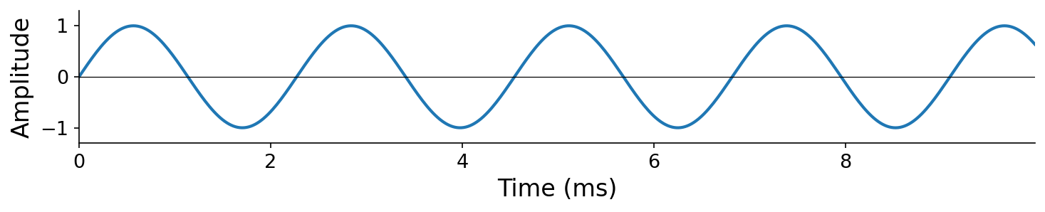
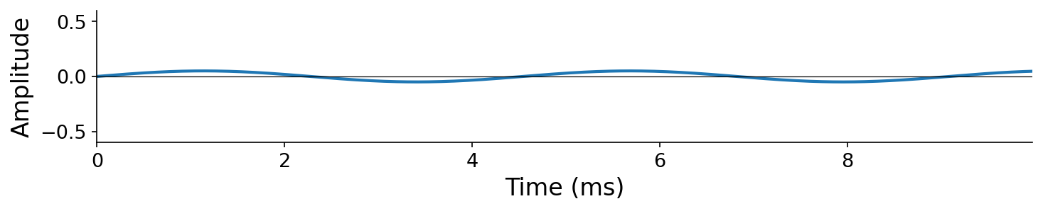
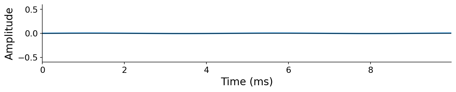
Amplitude determines loudness. Listen to the same 220 Hz tone at three different amplitudes:
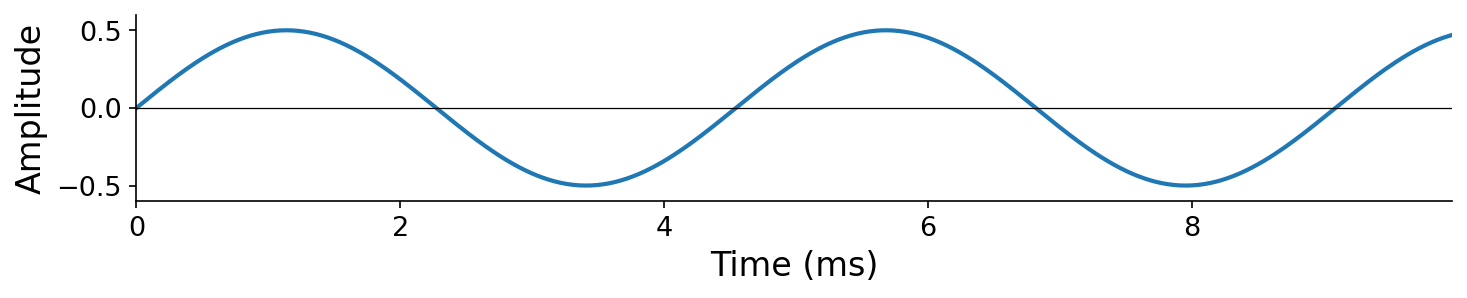
220 Hz sine, amplitude 0.5 Waveform at amplitude 0.5

220 Hz sine, amplitude 0.05 Waveform at amplitude 0.05

220 Hz sine, amplitude 0.005 Waveform at amplitude 0.005

The same frequency (220 Hz) at three amplitudes. The relationship between amplitude and our perception of “volume” is more nuanced than it appears here — we will formalize this when we study decibels.

Initial phase and instantaneous phase#

At a high level, phase characterizes our position within a cycle. In the basic sinusoid, phase appears in two forms:

  1. The initial phase \(\phi\) — a constant offset in radians that shifts the waveform’s starting point.

  2. The instantaneous phase \(\theta(t) = 2\pi f t + \phi = \omega t + \phi\) — the total phase of the sinusoid at time \(t\), in radians.

The instantaneous phase at time \(t\) equals the radians elapsed based on angular frequency \(\omega\) \(\frac{\text{radians}}{\text{second}}\) plus the initial offset \(\phi\) \(\text{radians}\). We can rewrite the basic sinusoid as \(x(t) = a \sin(\theta(t))\).

Example 1 (Instantaneous phase)

Consider our working example: \(f = 2\) Hz, \(\phi = \pi/2\). The angular frequency is \(\omega = 4\pi\) \(\frac{\text{radians}}{\text{second}}\), so \(\theta(t) = 4\pi t + \pi/2\). At a few specific times:

  • \(\theta(0) = \pi/2\) radians (the initial phase)

  • \(\theta(0.5) = 4\pi \cdot 0.5 + \pi/2 = 5\pi/2\) radians (one full period later)

  • \(\theta(1) = 4\pi \cdot 1 + \pi/2 = 9\pi/2\) radians (two full periods later)

Notice that \(\theta\) increases by \(2\pi\) radians each period — exactly one full cycle.

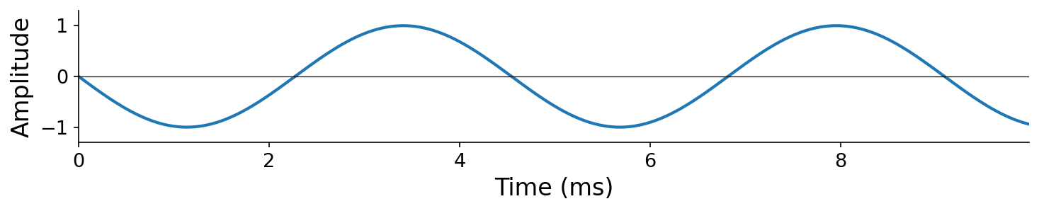
Our perception of phase differs from that of frequency and amplitude. Listen to a 220 Hz tone at three different initial phases:
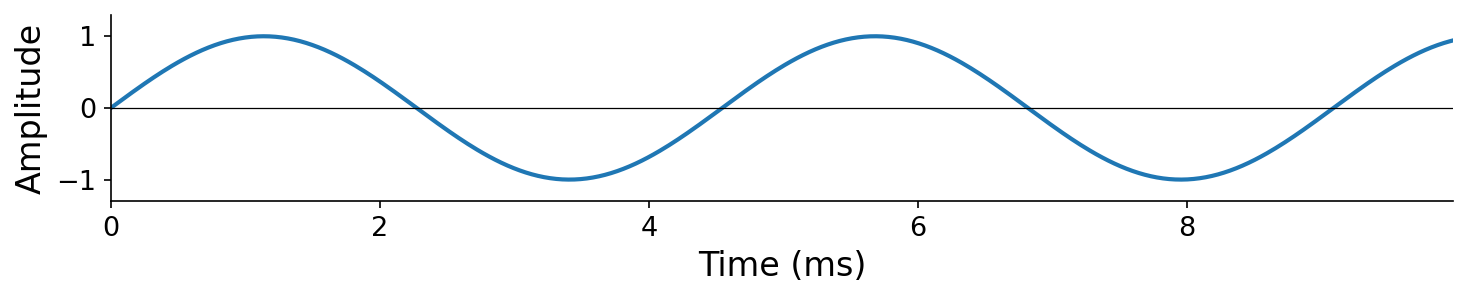
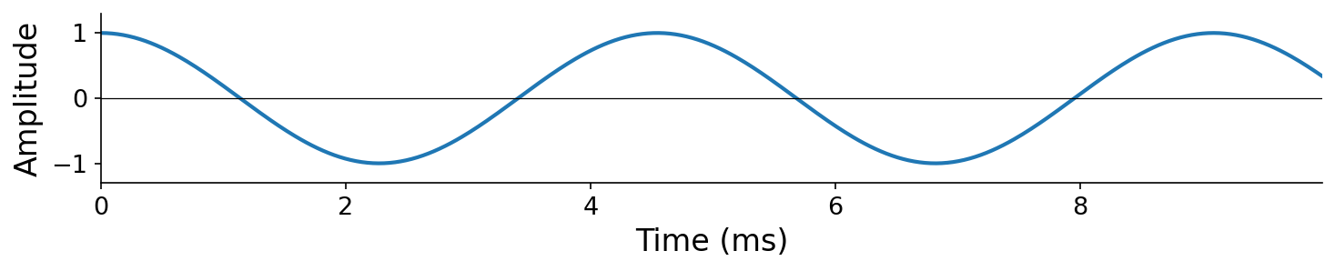
Phase = 0 Waveform at phase 0

Phase = pi/2 Waveform at phase pi/2

Phase = pi Waveform at phase pi

The same frequency (220 Hz) and amplitude at three initial phases. The waveforms are visually shifted in time, but they sound nearly identical.

Aside from slightly different “clicks” at the onset and offset of the waveform (caused by the signal’s value at the very first and last sample), these tones sound essentially the same. This is a general property of human hearing: we are largely insensitive to the absolute phase of a sound. This perceptual insensitivity will become important when we discuss additive synthesis below.

The interactive below puts all three parameters in one place. Drag the sliders and watch the waveform respond.

# hide
# no-output
from IPython.utils.capture import capture_output
with capture_output():
    %pip install -q plotly anywidget

import asyncio
import os
import numpy as np
import plotly.graph_objects as go
import ipywidgets as widgets
from IPython.display import Audio
import icm_plotly
from icm_plotly import RED, GOLD, STEEL, TEAL

Drag the sliders: the red curve is \(x(t) = a \sin(2 \pi f t + \phi)\), redrawn live. The gray curve keeps the starting parameters for reference, and the dashed teal lines mark one period \(t_0 = 1/f\). The audio card underneath always plays the current settings.

# hide
# autorun
T_MS = 20.0                             # window: 20 ms of signal
t = np.linspace(0.0, T_MS / 1000, 900)

A0, F0, PHI0 = 0.8, 220.0, 0.0          # the fixed reference parameters
sr = 44100
tt = np.arange(sr) / sr                  # one second of sample times
y_ref = A0 * np.sin(2 * np.pi * F0 * t + PHI0)

def period_marks(f, phi):
    # one period, bracketed from the first rising zero crossing
    start = ((-phi / (2 * np.pi)) % 1.0) / f
    return start, start + 1 / f

def figure():
    fig = go.Figure()
    fig.add_scatter(x=t * 1000, y=y_ref, mode="lines",
                    line=dict(color=STEEL, width=1.6))
    fig.add_scatter(x=t * 1000, y=y_ref, mode="lines",
                    line=dict(color=RED, width=2.2))
    for y in (A0, -A0):
        fig.add_scatter(x=[0, T_MS], y=[y, y], mode="lines",
                        line=dict(color=GOLD, width=1.2, dash="dash"))
    p0, p1 = period_marks(F0, PHI0)
    for x in (p0, p1):
        fig.add_scatter(x=[x * 1000, x * 1000], y=[-1.05, 1.05], mode="lines",
                        line=dict(color=TEAL, width=1.2, dash="dash"))
    fig.update_xaxes(range=[0, T_MS], title_text="Time (ms)", fixedrange=True)
    fig.update_yaxes(range=[-1.05, 1.05], title_text="Amplitude",
                     fixedrange=True)
    return fig

def controls(fig):
    amp = widgets.FloatSlider(description="Amplitude a", min=0, max=1,
                              value=A0, step=0.01)
    freq = widgets.FloatSlider(description="Frequency f (Hz)", min=110,
                               max=880, value=F0, step=5)
    phase = widgets.FloatSlider(description="Phase φ (rad)", min=0,
                                max=round(2 * np.pi, 2), value=PHI0, step=0.05)
    readout = widgets.HTML()

    # the defaults snapshot the arrays; the page's notebooks share one kernel
    def update(a, f, phi, t=t, readout=readout):
        p0, p1 = period_marks(f, phi)
        with fig.batch_update():
            fig.data[1].y = a * np.sin(2 * np.pi * f * t + phi)
            fig.data[2].y = [a, a]
            fig.data[3].y = [-a, -a]
            fig.data[4].x = [p0 * 1000, p0 * 1000]
            fig.data[5].x = [p1 * 1000, p1 * 1000]
        readout.value = (
            f"<span style='font-size:0.9em'>period t₀ = 1/f = "
            f"{1000 / f:.2f} ms &nbsp;·&nbsp; angular frequency "
            f"ω = 2πf ≈ {2 * np.pi * f:.0f} rad/s</span>"
        )

    widgets.interactive_output(update, {"a": amp, "f": freq, "phi": phase})

    # the audio card under the controls: the previous clip stays in place
    # while you drag (so the layout never jumps) and is swapped for the new
    # one when the pointer releases (keyboard nudges settle on a timer). It is
    # written through the Output's synced `outputs` trait, which works
    # outside a kernel message, where display() output has no destination
    out = widgets.Output()
    gate = icm_plotly.release_gate()   # pointer state: is a slider mid-drag?
    pending = []
    dirty = []

    def render(tt=tt, sr=sr):
        # loudness follows a, with a = 1 at -18 dBFS
        x = 0.125 * amp.value * np.sin(2 * np.pi * freq.value * tt + phase.value)
        x[:441] *= np.linspace(0, 1, 441)
        x[-441:] *= np.linspace(1, 0, 441)
        audio = Audio(x.astype(np.float32), rate=sr, normalize=False)
        data, metadata = get_ipython().display_formatter.format(audio)
        # one assignment swaps the old card for the new one in place, so
        # the page never shows an empty card and nothing shifts
        out.outputs = ({"output_type": "display_data",
                        "data": data, "metadata": metadata},)

    async def settle():
        await asyncio.sleep(0.25)
        pending.clear()
        if dirty and not gate.dragging:
            dirty.clear()
            render()

    def on_change(_):
        dirty.append(True)
        if pending:
            pending.pop().cancel()
        pending.append(asyncio.ensure_future(settle()))

    def on_release(change):
        if not change["new"] and dirty:
            if pending:
                pending.pop().cancel()
            dirty.clear()
            render()

    gate.observe(on_release, names="dragging")

    for s in (amp, freq, phase):
        s.observe(on_change, names="value")
    if not os.environ.get("ICM_BOOK_BUILD"):   # the build bakes no card
        render()
    return widgets.VBox([amp, freq, phase, readout, out, gate])

icm_plotly.show(figure, controls)
Amplitude a0.80
Frequency f (Hz)220.00
Phase φ (rad)0.00
period t₀ = 1/f = 4.55 ms  ·  angular frequency ω = 2πf ≈ 1382 rad/s