9.2 Convolution

In the previous section we met two difference equations with quite different behaviors,

\[\purple{y_1[n]} = \blue{x[n]} + \blue{x[n-1]}, \qquad \purple{y_2[n]} = \tfrac{1}{2}\blue{x[n]} - \tfrac{1}{2}\blue{x[n-1]}.\]

How might we generalize this idea? The trick is to write both filters in a single common format, attaching an explicit coefficient to every delayed term,

\[\begin{split} \begin{aligned} \purple{y_1[n]} &= \red{1} \cdot \blue{x[n]} &+ \red{1} \cdot \blue{x[n-1]}, \\ \purple{y_2[n]} &= \red{\tfrac{1}{2}} \cdot \blue{x[n]} &- \red{\tfrac{1}{2}} \cdot \blue{x[n-1]}. \end{aligned} \end{split}\]

The pattern is now clear. Each filter is a weighted sum of delayed copies of the input, and a filter is fully specified by its list of weights: \([1, 1]\) for the first and \([\tfrac{1}{2}, -\tfrac{1}{2}]\) for the second. Collecting the weights into a sequence \(\red{h}\), every filter of this form (of any length) can be written in a common format known as convolution.

Definition 26 (Convolution)

The convolution of a length-\(K\) filter \(\red{h}\) with a length-\(N\) signal \(\blue{x}\) is the signal

\[\purple{y[n]} = \sum_{k=0}^{K-1} \red{h[k]} \cdot \blue{x[n-k]}.\]

This operation is so common that it has its own notation, an asterisk:

\[\purple{y} = \red{h} * \blue{x}.\]

An example of convolution

Let us work a small example by hand. Take a short input \(\blue{x} = [1, 1, 1]\) (length \(N = 3\)) and a short filter \(\red{h} = [3, 2, 1]\) (length \(K = 3\)). Applying the definition, each output sample is a sum of products, remembering that any out-of-range sample of \(x\) is zero:

\[\begin{split} \begin{aligned} \purple{y[0]} &= \red{h[0]}\blue{x[0]} &&+ \red{h[1]}\blue{x[-1]} &&+ \red{h[2]}\blue{x[-2]} &&= 3 + 0 + 0 &&= 3, \\ \purple{y[1]} &= \red{h[0]}\blue{x[1]} &&+ \red{h[1]}\blue{x[0]} &&+ \red{h[2]}\blue{x[-1]} &&= 3 + 2 + 0 &&= 5, \\ \purple{y[2]} &= \red{h[0]}\blue{x[2]} &&+ \red{h[1]}\blue{x[1]} &&+ \red{h[2]}\blue{x[0]} &&= 3 + 2 + 1 &&= 6, \\ \purple{y[3]} &= \red{h[0]}\blue{x[3]} &&+ \red{h[1]}\blue{x[2]} &&+ \red{h[2]}\blue{x[1]} &&= 0 + 2 + 1 &&= 3, \\ \purple{y[4]} &= \red{h[0]}\blue{x[4]} &&+ \red{h[1]}\blue{x[3]} &&+ \red{h[2]}\blue{x[2]} &&= 0 + 0 + 1 &&= 1, \\ \purple{y[5]} &= \red{h[0]}\blue{x[5]} &&+ \red{h[1]}\blue{x[4]} &&+ \red{h[2]}\blue{x[3]} &&= 0 + 0 + 0 &&= 0. \end{aligned} \end{split}\]

Fig. 52 Convolving \(\blue{x} = [1,1,1]\) with \(\red{h} = [3,2,1]\) yields \(\purple{y} = [3,5,6,3,1]\). The output has five nonzero samples.

Notice that the output \(\purple{y} = [3, 5, 6, 3, 1]\) is longer than either input. In general, convolving a length-\(N\) signal with a length-\(K\) filter produces an output with \(N + K - 1\) nonzero samples. The convolution “spreads” the input out by the length of the filter.

You can watch convolution unfold as a sliding operation in the animation below, where a longer input signal is convolved with a filter. The filter slides across the input one sample at a time, and at each position the output sample is the sum of the overlapping products. Note that the filter appears reversed as it slides: this falls directly out of the definition, since the term \(\red{h[k]}\,\blue{x[n-k]}\) pairs the \(k\)-th filter coefficient with the input sample \(k\) steps back, so larger \(k\) reaches further into the past.

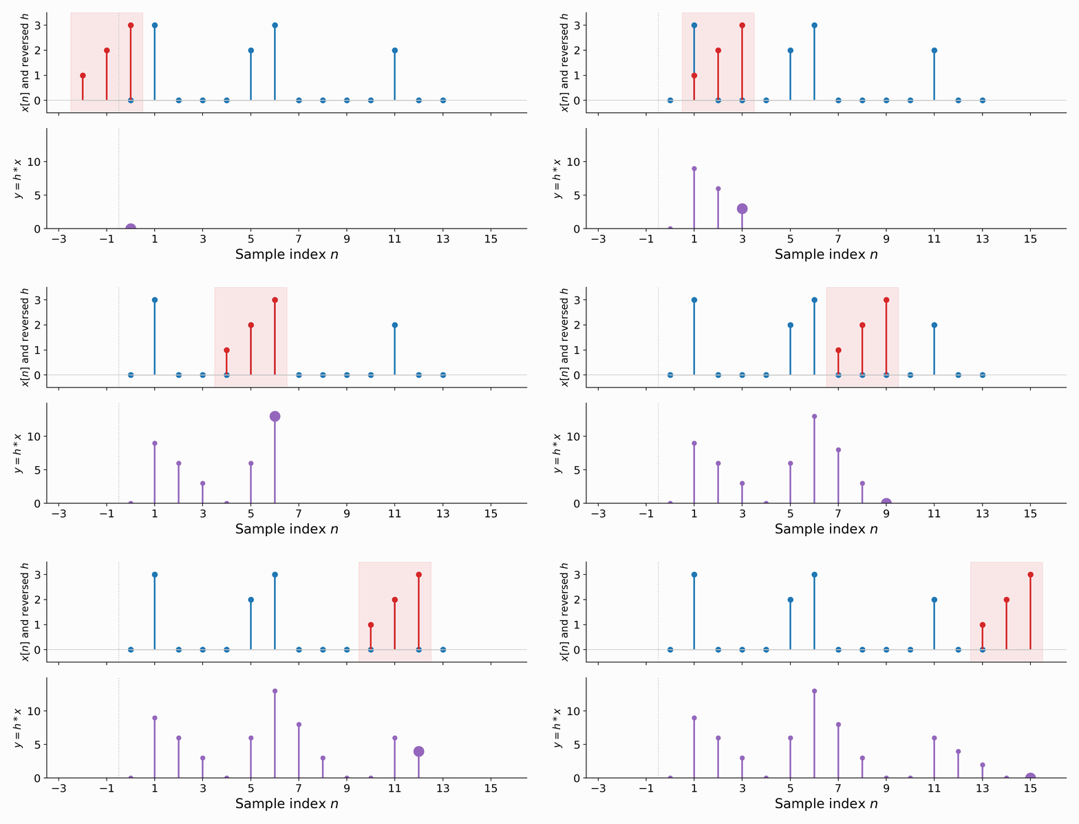
Fig. 53 Convolution as a sliding sum. The reversed filter \(\red{h}\) slides across the input \(\blue{x}\) one sample at a time, starting where it overlaps the assumed-zero samples before \(n = 0\). At each position, the overlapping products are summed to produce one output sample of \(\purple{y}\).

Commutativity of convolution

What happens if we swap the roles of \(\red{h}\) and \(\blue{x}\), convolving \(\blue{x} * \red{h}\) instead of \(\red{h} * \blue{x}\)? Reworking the same example with the roles reversed, so now the input is summed against the filter, gives

\[\begin{split} \begin{aligned} \purple{y[0]} &= \blue{x[0]}\red{h[0]} &&+ \blue{x[1]}\red{h[-1]} &&+ \blue{x[2]}\red{h[-2]} &&= 3 + 0 + 0 &&= 3, \\ \purple{y[1]} &= \blue{x[0]}\red{h[1]} &&+ \blue{x[1]}\red{h[0]} &&+ \blue{x[2]}\red{h[-1]} &&= 2 + 3 + 0 &&= 5, \\ \purple{y[2]} &= \blue{x[0]}\red{h[2]} &&+ \blue{x[1]}\red{h[1]} &&+ \blue{x[2]}\red{h[0]} &&= 1 + 2 + 3 &&= 6, \\ \purple{y[3]} &= \blue{x[0]}\red{h[3]} &&+ \blue{x[1]}\red{h[2]} &&+ \blue{x[2]}\red{h[1]} &&= 0 + 1 + 2 &&= 3, \\ \purple{y[4]} &= \blue{x[0]}\red{h[4]} &&+ \blue{x[1]}\red{h[3]} &&+ \blue{x[2]}\red{h[2]} &&= 0 + 0 + 1 &&= 1, \\ \purple{y[5]} &= \blue{x[0]}\red{h[5]} &&+ \blue{x[1]}\red{h[4]} &&+ \blue{x[2]}\red{h[3]} &&= 0 + 0 + 0 &&= 0. \end{aligned} \end{split}\]

which produces exactly the same output \([3, 5, 6, 3, 1]\). This is no accident. Convolution is commutative:

\[\red{h} * \blue{x} = \blue{x} * \red{h}.\]

In other words, it does not matter which signal we call the “filter” and which the “input”, the result is identical.

Other properties of convolution

Beyond commutativity, convolution has two more essential algebraic properties. We state them here and leave their proofs (a matter of manipulating the summation) as exercises.

Property 1 (Commutativity)

Convolution is commutative: \(\;a * b = b * a\).

Property 2 (Associativity)

Convolution is associative: \(\;a * (b * c) = (a * b) * c\).

Property 3 (Distributivity)

Convolution is distributive over addition: \(\;a * (b + c) = a * b + a * c\).

Associativity and commutativity have a practical consequence worth scrutinizing further. For a chain of convolutions like \(a * b * c\), computing in any order gives the same result, but some orders require far less work than others.

To see this, note that convolving a length-\(K\) filter with a length-\(N\) signal costs at least \(K \cdot N\) multiplications. Suppose \(a\), \(b\), and \(c\) have lengths \(A < B < C\). Then:

1. Computing \(a * (b * c)\) first convolves \(b * c\) (cost \(BC\), length \(B + C - 1\)), then convolves \(a\) with the result (cost \(A(B + C - 1)\)). The total is \(BC + AB + AC - A\).

2. Computing \((a * b) * c\) first convolves \(a * b\) (cost \(AB\), length \(A + B - 1\)), then convolves with \(c\) (cost \((A + B - 1)C\)). The total is \(AB + AC + BC - C\).

The two totals differ only in their final term: \(-A\) versus \(-C\). Since \(C > A\), the second ordering subtracts more and therefore costs less. The lesson is that when convolving several signals, it pays to combine the shorter ones first.

Implementing convolution

Convolution translates directly into code. A literal transcription of the definition uses two nested loops, one over the output index \(n\) and one over the filter index \(k\):

def convolve(x: np.ndarray, h: np.ndarray) -> np.ndarray:
    N, K = len(x), len(h)
    y = np.zeros(N + K - 1)
    for n in range(N + K - 1):
        for k in range(K):
            if 0 <= n - k < N:      # samples outside x are zero
                y[n] += h[k] * x[n - k]
    return y

The full runnable version, checked against NumPy’s np.convolve, is in code/convolve.py. The two nested loops make the cost plain: producing \(N + K - 1\) outputs, each a sum of up to \(K\) products, is an \(O(NK)\) computation. This is perfectly fine for the short filters behind simple difference equations. But as the input lengths \(N\) and \(K\) grow (sometimes hundreds of thousands of samples long in practical scenarios), the quadratic cost becomes a serious problem. We will return to this shortly with a dramatically faster approach.