import matplotlib
if not hasattr(matplotlib.RcParams, "_get"):
    matplotlib.RcParams._get = dict.get

9.8 Analyzing filters

We have looked at filters both in their low-level implementation (difference equations, convolution) and in their high-level behavior (sculpting in frequency domain, convolution theorem). But how might we connect the two? We have two directions to worry about. Given a filter (its difference equation or impulse response), how do analyze its frequency response, to know what it will do to a sound? And conversely, given a desired frequency response, how do we design a filter that achieves it? There are entire textbooks written on these questions. In this book, we will consider filter design as explicitly out of scope, and present only a cursory empirical perspective on filter analysis here.

The empirical idea is simple and follows directly from what an LTI filter does: it scales each frequency by some amount. So to probe the response at a given frequency, we feed the filter a pure sinusoid at that frequency and measure how much the output’s amplitude changed.

Let’s start by looking at a simple FIR filter that we discussed previously, \(y[n] = x[n] + x[n-1]\), at three telling frequencies: DC (\(0\) Hz), a quarter of the sample rate (\(f_s/4\)), and the Nyquist frequency (\(f_s/2\)). At each, we write down the sampled cosine \(x[n] = \cos(2\pi f n / f_s)\) and push it through the difference equation:

\[\begin{split} \begin{aligned} f &= 0: \quad &x = [1, 1, 1, 1, \ldots], && y = [1, 2, 2, 2, \ldots], && \max|y| = 2, \\ f &= \tfrac{f_s}{4}: \quad &x = [1, 0, -1, 0, \ldots], && y = [1, 1, -1, -1, \ldots], && \max|y| = 1, \\ f &= \tfrac{f_s}{2}: \quad &x = [1, -1, 1, -1, \ldots], && y = [1, 0, 0, 0, \ldots], && \max|y| = 0. \end{aligned} \end{split}\]

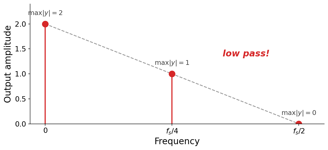
Fig. 58 Probing \(y[n] = x[n] + x[n-1]\) by hand at three frequencies. The output amplitude falls from \(2\) at DC to \(0\) at Nyquist. Just three points are enough to recognize the shape: a low-pass filter.

Three points already reveal the trend, and confirm by measurement what we guessed from the filter’s smoothing effect earlier: it is a low-pass. To fill in the whole curve, we automate the same procedure, sweeping the probe frequency across the full range and recording the output amplitude at each:

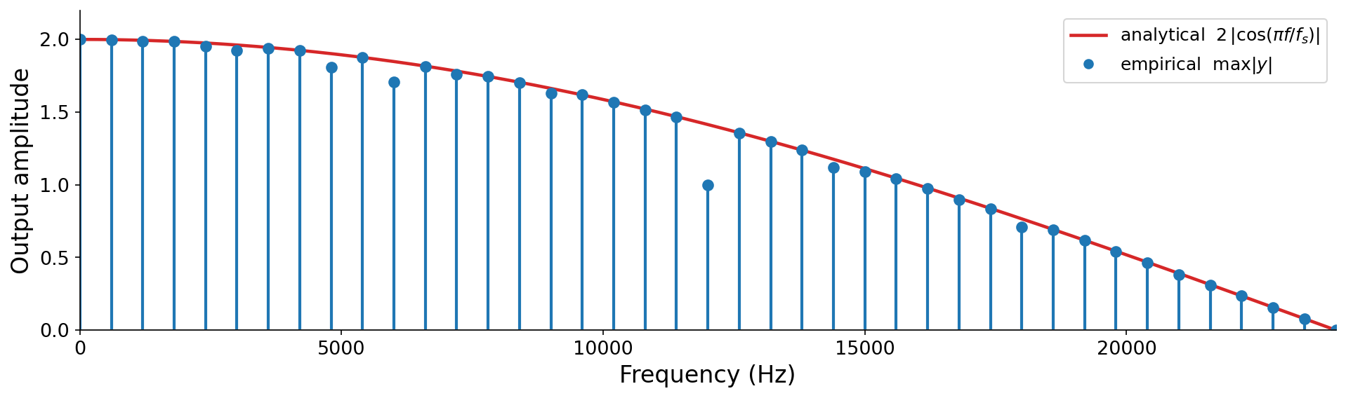
Fig. 59 The empirically measured frequency response of \(y[n] = x[n] + x[n-1]\) (blue stems), obtained by probing with sinusoids at forty-one frequencies including exactly \(f_s/4\) and \(f_s/2\). The probe points at those two frequencies read \(1\) and \(0\), matching our hand calculations above.

Sweeping across the whole band confirms the low-pass shape unmistakably: the response falls smoothly from a gain of \(2\) at DC to \(0\) at Nyquist, passing through exactly \(1\) at \(f_s/4\) and \(0\) at Nyquist as we computed by hand. Look closely, though, and a few probe points sit slightly below the otherwise smooth trend. These outliers are an artifact of our crude amplitude estimate. We take a sinusoid’s amplitude to be its largest sample, \(\max|y|\), but the true peak of the underlying continuous wave usually falls between two samples, so the largest sample we happen to catch undershoots it. The \(f_s/4\) point is one such case, reading exactly \(1\), below the sinusoid’s true peak.

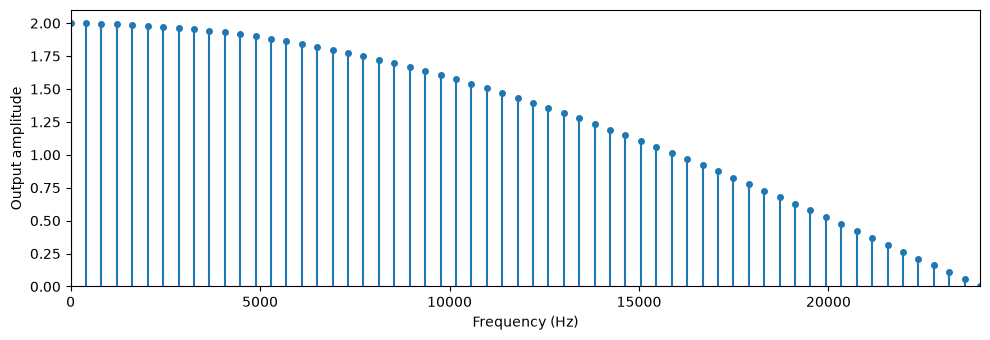
This same response can be derived analytically instead of measured, giving the exact closed form \(2\,|\cos(\pi f / f_s)|\) (the red curve above). The derivation is beyond our scope, but interested readers can follow it through Smith’s mathematical sine-wave analysis and rederiving the frequency response [Smi07b]. Because the analytical formula gives the true peak directly, free of the between-samples problem, it always upper-bounds the empirical measurement, which is why every probe point lands on or just below it. The empirical method, by contrast, requires no derivation at all and works for any filter you can run. You can measure the response of your own filters, including ones you invent, in the following example:

# hide
import numpy as np
import matplotlib.pyplot as plt

F_S = 48000


def frequency_response(h, num_probes=60):
    """Measure a filter's frequency response empirically.

    The filter is the FIR filter whose impulse response is ``h``. We probe it
    with a pure sinusoid at each of ``num_probes`` frequencies and estimate the
    output amplitude as its largest sample, ``max|y|``. Because the true peak of
    the continuous output usually falls between samples, this slightly
    under-estimates the response at some frequencies (a lower bound).
    """
    h = np.asarray(h, dtype=float)
    freqs = np.linspace(0, F_S / 2, num_probes)
    n = np.arange(int(0.25 * F_S))            # a quarter second per probe
    amps = []
    for f in freqs:
        x = np.cos(2 * np.pi * f * n / F_S)   # probe sinusoid
        y = np.convolve(x, h, mode="valid")   # steady-state output (drop warm-up/tail edges)
        amps.append(np.max(np.abs(y)))        # amplitude estimate = largest sample

    plt.figure(figsize=(10, 3.5))
    ml, sl, bl = plt.stem(freqs, amps)
    plt.setp(ml, color="C0", markersize=4)
    plt.setp(sl, color="C0")
    plt.setp(bl, visible=False)
    plt.xlabel("Frequency (Hz)")
    plt.ylabel("Output amplitude")
    plt.xlim(0, F_S / 2)
    plt.ylim(bottom=0)
    plt.tight_layout()
    plt.show()

# An impulse response fully describes an LTI filter. Enter one here and see the
# frequency response it produces, then try the others below or design your own.
h = [1, 1]

# More to try (uncomment one line at a time):
# h = [1, -1]        # a difference (passes the highs)
# h = [1, 0, 0, 1]   # x[n] + x[n-3] (a comb filter, with notches)
# h = [0.2] * 5      # a five-tap moving average (a stronger low pass)

frequency_response(h)

Note

We have only measured the amplitude response, how much each frequency is scaled. LTI filters also affect phase, shifting each frequency in time, described by the filter’s phase response \(\angle H(\omega)\). Phase matters whenever filtered signals are mixed back together, where it governs constructive and destructive interference, and it can be manipulated creatively (a guitar “phaser” is one example). An all-pass filter is designed to leave every amplitude untouched while altering only the phase.