9.7 Filter types#
LTI filters are often categorized by the shape of their frequency response, that is, by which bands of frequencies they pass and which they reject. A handful of shapes are so common that they have standard names. We start with their idealized forms, drawn as perfectly sharp “brick-wall” responses:

Fig. 56 The four canonical filter shapes, drawn as idealized “brick-wall” magnitude responses. The passband (shaded) is the range of frequencies that pass through, the stopband is the range that is rejected, and the cutoff frequency \(f_C\) marks the boundary (placed at the center of the band for the band-pass and band-stop).#
A low-pass filter passes low frequencies and rejects those above its cutoff. Rolling off a sound’s upper frequencies to make it darker or muffled is a low-pass.
A high-pass filter does the opposite, passing high frequencies and rejecting those below its cutoff. Removing low-frequency rumble is a high-pass.
A band-pass filter passes a band of frequencies around a center frequency and rejects everything else. A telephone or a “lo-fi” effect is roughly band-pass.
A band-stop filter, also called a notch, is the inverse: it rejects a band and passes everything else. Removing a single offending hum frequency is a notch.
To hear the difference, here is the same burst of white noise (which contains every frequency in equal measure) passed through each of the four filter types. Real filters are not the brick walls drawn above, so some sound leaks through the stopbands, but the character of each is unmistakable:
Original white noise (all frequencies)
The unfiltered source: white noise, with equal energy at every frequency.
From ideal to real#
Real digital filters cannot achieve those perfectly vertical brick-wall edges. An actual low-pass response rolls off gradually, and this forces us to be precise about what “cutoff” even means. By convention, the cutoff frequency \(f_C\) is the point where the response has fallen to some amplitude threshold (often \(-6\) dB or half the amplitude), and the region between the passband and the stopband, where the response slides from \(-6\) dB down to some “fully rejected” level like \(-60\) dB, is called the transition band:
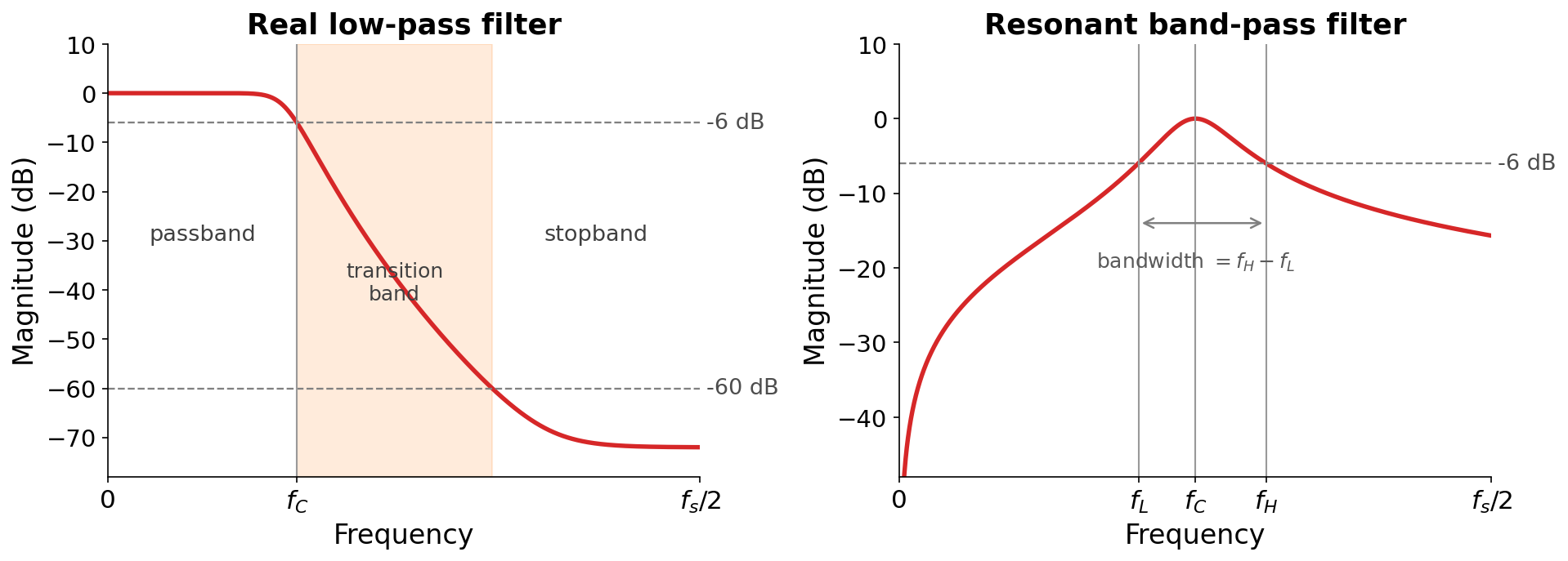
Fig. 57 Left: a real low-pass filter. The cutoff frequency \(f_C\) is where the response crosses \(-6\) dB, and the transition band (shaded) is the gradual slide from there down to the stopband (here \(-60\) dB). Right: a real band-pass filter, whose passband edges \(f_L\) and \(f_H\) are the two \(-6\) dB crossings; the bandwidth is \(f_H - f_L\).#
The steepness of the transition band is one of the main things filter design trades off against cost: a sharper transition needs a higher-order filter and more computation. For a band-pass filter, the two \(-6\) dB crossings \(f_L\) and \(f_H\) bracket the passband, and their difference is the bandwidth, \(f_H - f_L\). A narrow bandwidth means a more selective, sharply-tuned filter. This selectivity is quantified by the filter’s quality factor, or \(Q\):
A high \(Q\) means a narrow, resonant peak (very selective), while a low \(Q\) means a broad, gentle one. \(Q\) is the “resonance” knob on a synthesizer filter, and we will hear its effect in the subtractive-synthesis examples below.