5.1 A review of the complex plane

import matplotlib
if not hasattr(matplotlib.RcParams, "_get"):
    matplotlib.RcParams._get = dict.get

5.1 A review of the complex plane#

Sound exists in the real world, so why are we suddenly invoking the complex plane, with its “imaginary” numbers? The answer is that the complex plane is an exceptionally convenient analytical tool for modeling periodic phenomena, even thoroughly real-world ones like audio signals. The key connection, which we will make precise shortly, is that rotation is the fundamental periodic phenomenon, and multiplication in the complex plane models rotation [McF23].

This book assumes complex numbers as background knowledge, but we revisit the essentials here in case you are rusty, which is perfectly fine.

Tip

In this book, prefer to think of \(j\) as an analytical tool for better understanding real-valued signals, rather than as an “imaginary number”. This framing demystifies much of what follows.

We write the imaginary unit as \(j = \sqrt{-1}\), rather than \(i\), following the convention in engineering and digital signal processing (where \(i\) often denotes other quantities, such as electric current). A complex number \(z\) can be written in rectangular form (also called Cartesian form) as a pair of real coordinates \((x, y)\):

\[z = x + jy,\]

where \(x\) is the real part and \(y\) is the imaginary part.

Two complex numbers in rectangular form are added componentwise, and multiplied using the single rule \(j^2 = -1\). We collect both operations here for reference:

Definition 14 (Complex addition and multiplication (rectangular form))

For \(z_1 = x_1 + j y_1\) and \(z_2 = x_2 + j y_2\),

\[z_1 + z_2 = (x_1 + x_2) + j(y_1 + y_2),\]

\[z_1 \cdot z_2 = (x_1 x_2 - y_1 y_2) + j(x_1 y_2 + x_2 y_1).\]

Addition simply adds the real and imaginary parts separately. The multiplication rule looks more involved, but it follows from expanding the product like any pair of binomials and then applying \(j^2 = -1\):

\[\begin{split} \begin{aligned} z_1 \cdot z_2 &= (x_1 + j y_1)(x_2 + j y_2) \\ &= x_1 x_2 + j x_1 y_2 + j y_1 x_2 + j^2 y_1 y_2 \\ &= x_1 x_2 + j x_1 y_2 + j y_1 x_2 - y_1 y_2 && (j^2 = -1) \\ &= (x_1 x_2 - y_1 y_2) + j(x_1 y_2 + x_2 y_1). \end{aligned} \end{split}\]

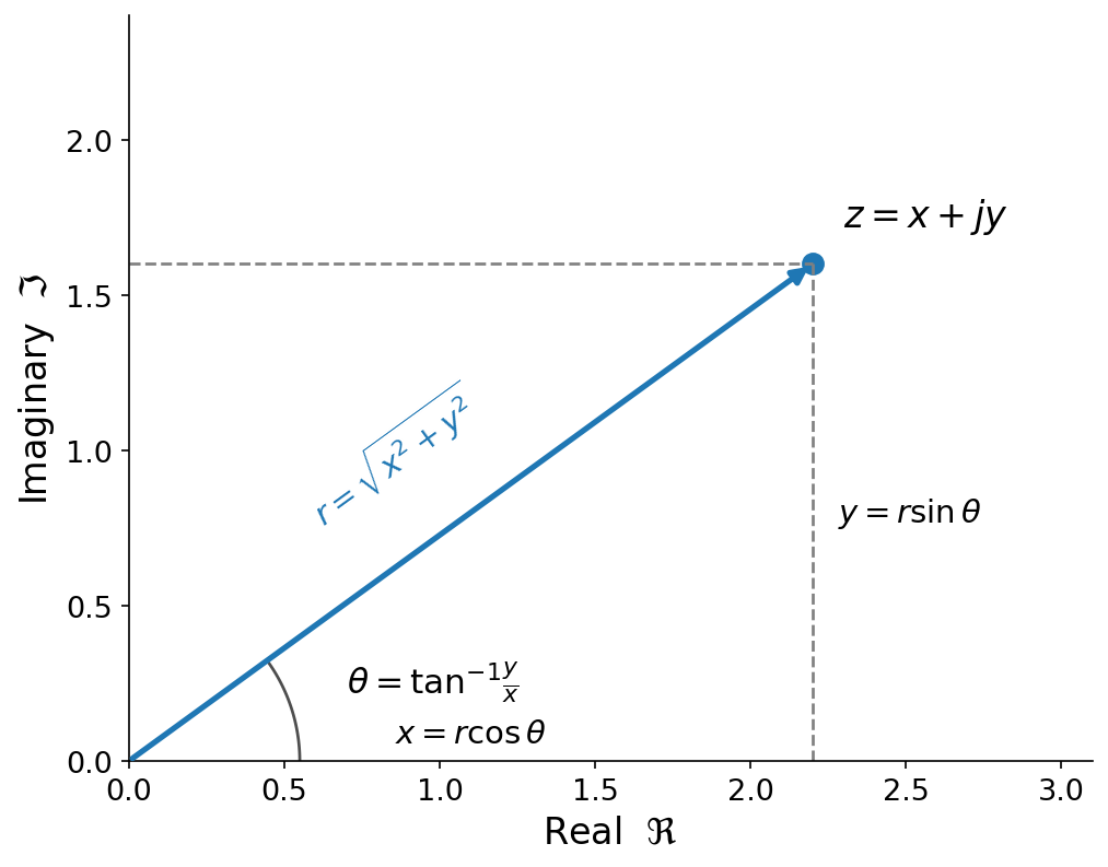
A complex number can equivalently be written in polar form as a pair \((r, \theta)\), giving its magnitude (distance from the origin) \(r\) and its angle \(\theta\) from the real axis. Rectangular and polar are just two coordinate systems for the same point, related by basic trigonometry:

\[ r = \sqrt{x^2 + y^2}, \qquad \theta = \tan^{-1}\!\left(\frac{y}{x}\right), \]

and in the other direction,

\[ x = r\cos\theta, \qquad y = r\sin\theta. \]

A complex number z = x + jy plotted as a point in the first quadrant, with the real axis horizontal and the imaginary axis vertical. A vector from the origin to z has length r and makes angle theta with the real axis. Dashed lines show the projections x = r cos theta and y = r sin theta. — Fig. 18 A complex number \(z\) in the complex plane. Rectangular form \((x, y)\) gives its horizontal and vertical coordinates. Polar form \((r, \theta)\) gives its distance from the origin and its angle from the real axis.#

Polar form is especially convenient for multiplication, where magnitudes multiply and angles add. For \(z_1 = (r_1, \theta_1)\) and \(z_2 = (r_2, \theta_2)\) in polar form,

\[z_1 \cdot z_2 = (r_1 r_2, \; \theta_1 + \theta_2).\]

This is the precise sense in which multiplication models rotation: multiplying by a number of magnitude 1 and angle \(\theta\) rotates a point by \(\theta\) without changing its distance from the origin. Hold onto this idea, as it is the engine of everything that follows.

The widget below puts two complex numbers side by side. Drag their magnitudes and angles, and watch the magnitudes multiply and the angles add.

# hide
# no-output
from IPython.utils.capture import capture_output
with capture_output():
    %pip install -q plotly anywidget

import numpy as np
import plotly.graph_objects as go
from plotly.subplots import make_subplots
import ipywidgets as widgets
import icm_plotly
from icm_plotly import RED, BLUE, GOLD, IRON, TEAL, STEEL

Drag the four sliders. The red and blue arrows are \(z_1 = (r_1, \theta_1)\) and \(z_2 = (r_2, \theta_2)\), and the gold arrow is their product \(z_1 z_2\). Watch the angles add and the magnitudes multiply. The gray circle marks magnitude 1: multiplying by a number on it only rotates.

# hide
# autorun
R1_0, A1_0, R2_0, A2_0 = 1.2, 35.0, 1.0, 55.0    # starting parameters

CIRC = np.linspace(0.0, 2 * np.pi, 361)

def vec(r, deg):
    a = np.radians(deg)
    return r * np.cos(a), r * np.sin(a)

def arc(deg, radius, n=120):
    a = np.linspace(0.0, np.radians(deg), n)
    return radius * np.cos(a), radius * np.sin(a)

def figure():
    fig = go.Figure()
    fig.add_scatter(x=np.cos(CIRC), y=np.sin(CIRC), mode="lines",
                    line=dict(color=STEEL, width=1.4, dash="dot"))
    for deg, radius, color in ((A1_0, 0.34, RED), (A2_0, 0.50, BLUE),
                               (A1_0 + A2_0, 0.66, GOLD)):
        ax, ay = arc(deg, radius)
        fig.add_scatter(x=ax, y=ay, mode="lines",
                        line=dict(color=color, width=1.4, dash="dot"))
    for r, deg, color, width in ((R1_0, A1_0, RED, 2.6),
                                 (R2_0, A2_0, BLUE, 2.6),
                                 (R1_0 * R2_0, A1_0 + A2_0, GOLD, 3.4)):
        vx, vy = vec(r, deg)
        fig.add_scatter(x=[0, vx], y=[0, vy], mode="lines+markers",
                        line=dict(color=color, width=width),
                        marker=dict(color=color, size=[1, 10]))
    # a tall figure with a narrow x domain keeps the plotting area square, so
    # the equal-aspect constraint does not stretch the frame sideways
    fig.update_layout(height=520)
    fig.update_xaxes(domain=[0.24, 0.76], range=[-2.6, 2.6], title_text="Re",
                     fixedrange=True, scaleanchor="y", scaleratio=1)
    fig.update_yaxes(range=[-2.6, 2.6], title_text="Im", fixedrange=True)
    return fig

def controls(fig):
    r1 = widgets.FloatSlider(description="$r_1$", min=0.2, max=1.5, value=R1_0,
                             step=0.05)
    a1 = widgets.FloatSlider(description=r"$\theta_1$ (deg)", min=-180, max=180,
                             value=A1_0, step=5)
    r2 = widgets.FloatSlider(description="$r_2$", min=0.2, max=1.5, value=R2_0,
                             step=0.05)
    a2 = widgets.FloatSlider(description=r"$\theta_2$ (deg)", min=-180, max=180,
                             value=A2_0, step=5)
    readout = widgets.HTML()

    # the defaults snapshot the helpers; the page's notebooks share one kernel
    def update(r1, a1, r2, a2, vec=vec, arc=arc, readout=readout):
        with fig.batch_update():
            for i, (deg, radius) in enumerate(((a1, 0.34), (a2, 0.50),
                                               (a1 + a2, 0.66))):
                fig.data[1 + i].x, fig.data[1 + i].y = arc(deg, radius)
            for i, (r, deg) in enumerate(((r1, a1), (r2, a2),
                                          (r1 * r2, a1 + a2))):
                vx, vy = vec(r, deg)
                fig.data[4 + i].x, fig.data[4 + i].y = [0, vx], [0, vy]
        x1, y1 = vec(r1, a1)
        x2, y2 = vec(r2, a2)
        zero = lambda v: 0.0 if abs(v) < 0.005 else v   # no "-0.00" readouts
        x1, y1, x2, y2 = zero(x1), zero(y1), zero(x2), zero(y2)
        px, py = zero(x1 * x2 - y1 * y2), zero(x1 * y2 + x2 * y1)
        def cx(x, y):   # x + yj, set like the chapter's formulas
            sign = "+" if y >= 0 else "&minus;"
            return f"{x:.2f}".replace("-", "&minus;") + f" {sign} {abs(y):.2f}<i>j</i>"

        readout.value = (
            f"<span style='font-size:0.9em'>"
            f"<i>z</i><sub>1</sub> = {cx(x1, y1)} &nbsp;·&nbsp; "
            f"<i>z</i><sub>2</sub> = {cx(x2, y2)}<br>"
            f"<i>z</i><sub>1</sub><i>z</i><sub>2</sub> = {cx(px, py)} &nbsp;·&nbsp; "
            f"<i>r</i><sub>1</sub><i>r</i><sub>2</sub> = {r1 * r2:.2f} &nbsp;·&nbsp; "
            f"<i>&theta;</i><sub>1</sub> + <i>&theta;</i><sub>2</sub> = {a1 + a2:.0f}&deg;"
            f"</span>")

    widgets.interactive_output(update, {"r1": r1, "a1": a1, "r2": r2, "a2": a2})
    return widgets.VBox([r1, a1, r2, a2, readout])

icm_plotly.show(figure, controls)

Finally, polar form connects back to rectangular form through one of the most important identities in all of mathematics, Euler’s formula:

\[e^{j\theta} = \cos\theta + j\sin\theta.\]

Reading it as a complex number, \(e^{j\theta}\) has real part \(\cos\theta\) and imaginary part \(\sin\theta\), so it is exactly the point on the unit circle at angle \(\theta\). A general complex number in polar form is therefore \(z = r e^{j\theta}\).