import matplotlib
if not hasattr(matplotlib.RcParams, "_get"):
    matplotlib.RcParams._get = dict.get

8.1 Issue 1: Finite signals

The Fourier transform is defined over infinitely long signals \(x(t) : \mathbb{R} \to \mathbb{R}\). But what if we only have a signal of some finite duration \(T\), defined on \([0, T)\)? Or, more generally, what if we want the frequency content of just a segment of a longer signal, defined on \([a, b]\)?

We already saw the key trick in Chapter 7 when we analyzed sampling. There we learned two useful strategies that we will apply here: (1) multiplying a continuous signal by a specially-shaped discontinuous one lets us model discrete phenomena, and (2) the Fourier transform of a discontinuous signal is perfectly well defined.

Windowing

To leverage a similar trick here, we first define a window function \(w_{a,b}(t)\). In general, a window is any function that is zero outside the interval of interest \([a, b]\) and non-negative within it:

\[\begin{split} w_{a,b}(t) \; \begin{cases} \geq 0 & \text{if } a \leq t \leq b, \\ = 0 & \text{otherwise.} \end{cases} \end{split}\]

The specific shape of the window inside \([a, b]\) is a design choice, and different shapes trade off different properties (as we will see shortly). The simplest choice is the rectangular window, which is exactly 1 on the interval and 0 outside:

\[\begin{split} \text{Rect}_{a,b}(t) = \begin{cases} 1 & \text{if } a \leq t \leq b, \\ 0 & \text{otherwise.} \end{cases} \end{split}\]

The idea is that a finite signal defined on \([a, b]\) can be viewed as an infinitely long signal multiplied by a corresponding rectangular window. Multiplying zeroes out everything outside \([a, b]\) and leaves the signal untouched inside it. The figure below shows the effect in both domains, using the same running example as Chapter 7, \(x(t) = \sin(2\pi t) + \sin(2\pi 2 t)\):

Fig. 42 Windowing a signal to a finite interval, viewed in both domains. Multiplying \(x(t)\) by the rectangular window \(\text{Rect}_{a,b}(t)\) (top) has a side effect in the frequency domain (bottom): each sharp spectral line of \(|X(\omega)|\) is smeared into a lobe, a phenomenon called spectral leakage.

Windowing was not free. Comparing the bottom-left and bottom-right panels, the sharp spectral spikes of the original signal have been smeared into lobes. This blurring is called spectral leakage: energy from each true frequency “leaks” into neighboring frequencies. We can still make out the basic shape of the spectrum, with peaks near the true frequencies of 1 and 2 Hz, but it is no longer exact.

Note

Leakage comes from the window’s own spectrum (the middle panel), which is a sinc function rather than a single spike. As we noted in Chapter 7, multiplication in time is convolution in frequency, so the true spectrum gets convolved with (smeared by) the window’s sinc.

Spectral leakage is the price of analyzing a finite slice of time, and it is unavoidable. However, we can potentially mitigate it by using a window whose own spectrum is better behaved than the rectangular window’s sinc. The abrupt jumps at the edges of the rectangular window are what create its strong side lobes; a window that instead tapers smoothly to zero at both ends has a much more compact spectrum. A common choice is the Hann window, a raised cosine that rises from zero at \(a\) to a peak at the center and back to zero at \(b\):

\[\begin{split} \text{Hann}_{a,b}(t) = \begin{cases} \dfrac{1}{2}\left[1 - \cos\!\left(2\pi\,\dfrac{t - a}{b - a}\right)\right] & \text{if } a \leq t \leq b, \\[2mm] 0 & \text{otherwise.} \end{cases} \end{split}\]

Repeating the same experiment with a Hann window in place of the rectangular one, the leakage is visibly reduced. The window’s spectrum (middle) has far smaller side lobes, so the windowed spectrum (bottom right) concentrates each component’s energy more tightly around its true frequency:

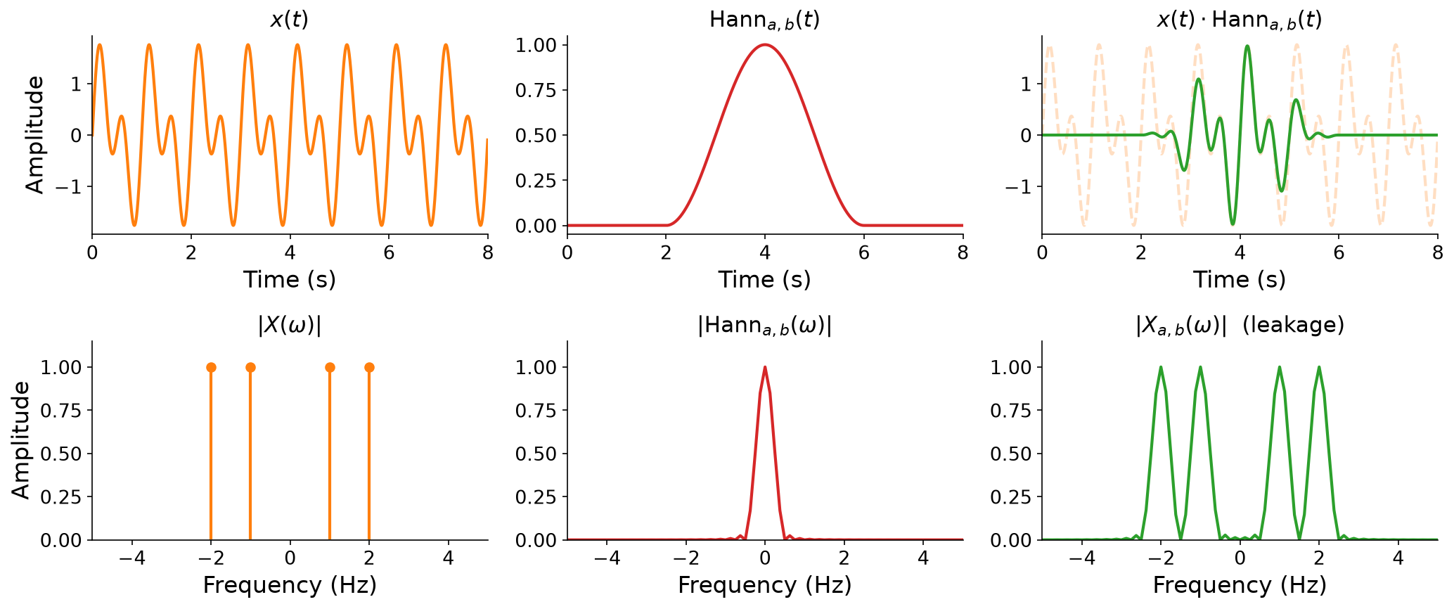
Fig. 43 The same windowing experiment with a Hann window. Compared to the rectangular window, the Hann window’s spectrum (middle) has much smaller side lobes, so its spectral leakage (bottom right) is more contained, at the cost of a slightly wider central lobe.

We will revisit other implications of windowing, including this central-lobe-versus-side-lobe tradeoff, when we study frame-based processing in Chapter 10. For now, we’ll assume that we’re applying rectangular windows.

The widget below runs the same experiment at any window length. Drag the length, switch between the two shapes, and watch the peaks widen and the side lobes rise and fall.

# hide
# no-output
from IPython.utils.capture import capture_output
with capture_output():
    %pip install -q plotly anywidget

import numpy as np
import plotly.graph_objects as go
from plotly.subplots import make_subplots
import ipywidgets as widgets
import icm_plotly
from icm_plotly import RED, BLUE, GOLD, IRON, TEAL, STEEL

Drag the window length and switch the shape. On the left, the gold curve is the window and the red curve is what the transform actually sees. On the right is the resulting amplitude spectrum in decibels, with the two true frequencies marked in gray. A shorter window widens every peak, and the Hann window trades a wider peak for much smaller side lobes.

# hide
# autorun
T0, SHAPE0 = 4.0, "Rectangular"     # starting parameters

SR_A = 200.0                        # analysis rate for the running example
T_TOT = 8.0
TA = np.arange(int(T_TOT * SR_A)) / SR_A
X = np.sin(2 * np.pi * TA) + np.sin(2 * np.pi * 2 * TA)
NFFT = 8192
FREQS = np.fft.rfftfreq(NFFT, 1 / SR_A)
MASK = FREQS <= 5.0

def window(T, shape):
    w = np.zeros_like(TA)
    inside = TA < T
    if shape == "Hann":
        w[inside] = 0.5 * (1 - np.cos(2 * np.pi * TA[inside] / T))
    else:
        w[inside] = 1.0
    return w

def spectrum(T, shape):
    mag = np.abs(np.fft.rfft(X * window(T, shape), NFFT))[MASK]
    return 20 * np.log10(np.maximum(mag / mag.max(), 1e-4))

def figure():
    fig = make_subplots(rows=1, cols=2, horizontal_spacing=0.13)
    w0 = window(T0, SHAPE0)
    fig.add_scatter(x=TA, y=X, mode="lines",
                    line=dict(color=STEEL, width=1.2), row=1, col=1)
    fig.add_scatter(x=TA, y=2.2 * w0, mode="lines",
                    line=dict(color=GOLD, width=1.8, dash="dash"),
                    row=1, col=1)
    fig.add_scatter(x=TA, y=X * w0, mode="lines",
                    line=dict(color=RED, width=1.6), row=1, col=1)
    fig.add_scatter(x=[1, 1, None, 2, 2, None], y=[-82, 4, None, -82, 4, None],
                    mode="lines", line=dict(color=STEEL, width=1.2, dash="dot"),
                    row=1, col=2)
    fig.add_scatter(x=FREQS[MASK], y=spectrum(T0, SHAPE0), mode="lines",
                    line=dict(color=BLUE, width=1.6), row=1, col=2)
    fig.update_xaxes(range=[0, T_TOT], title_text="Time (s)",
                     fixedrange=True, row=1, col=1)
    fig.update_yaxes(range=[-2.6, 2.6], title_text="Amplitude",
                     fixedrange=True, row=1, col=1)
    fig.update_xaxes(range=[0, 5], title_text="Frequency (Hz)",
                     fixedrange=True, row=1, col=2)
    fig.update_yaxes(range=[-82, 4], title_text="Magnitude (dB)",
                     fixedrange=True, row=1, col=2)
    return fig

def controls(fig):
    length = widgets.FloatSlider(description="Window length $T$ (s)", min=0.5,
                                 max=8.0, value=T0, step=0.1)
    shape = widgets.Dropdown(description="Window shape",
                             options=["Rectangular", "Hann"], value=SHAPE0)
    readout = widgets.HTML()

    # the defaults snapshot the arrays; the page's notebooks share one kernel
    def update(T, shape, X=X, window=window, spectrum=spectrum,
               readout=readout):
        w = window(T, shape)
        with fig.batch_update():
            fig.data[1].y = 2.2 * w
            fig.data[2].y = X * w
            fig.data[4].y = spectrum(T, shape)
        readout.value = (f"<span style='font-size:0.9em'><i>T</i> = {T:.1f} s "
                         f"&nbsp;·&nbsp; bin spacing 1/<i>T</i> = {1 / T:.2f} Hz"
                         f"</span>")

    widgets.interactive_output(update, {"T": length, "shape": shape})
    return widgets.VBox([length, shape, readout])

icm_plotly.show(figure, controls)

Window length \(T\) (s)4.00

Window shapeRectangular

T = 4.0 s  ·  bin spacing 1/T = 0.25 Hz

The windowed Fourier transform

Setting aside leakage, rectangular windowing gives us exactly what we wanted. To keep the algebra compact, let \(x_{a,b}(t) = x(t) \cdot \text{Rect}_{a,b}(t)\) denote the windowed signal. Splitting the Fourier transform at the window edges \(a\) and \(b\) gives three pieces:

\[\begin{split} \begin{aligned} \hat{X}(\omega) &= \int_{-\infty}^{\infty} x_{a,b}(t)\, e^{-j\omega t}\, dt \\ &= \int_{-\infty}^{a} x_{a,b}(t)\, e^{-j\omega t}\, dt + \int_{a}^{b} x_{a,b}(t)\, e^{-j\omega t}\, dt + \int_{b}^{\infty} x_{a,b}(t)\, e^{-j\omega t}\, dt \\ &= 0 + \int_{a}^{b} x_{a,b}(t)\, e^{-j\omega t}\, dt + 0 \\ &= \int_{a}^{b} x(t)\, e^{-j\omega t}\, dt. \end{aligned} \end{split}\]

The two outer integrals vanish because the window is zero outside \([a, b]\). In the surviving middle integral over \([a, b]\), the window is always one, so \(x_{a,b}(t) = x(t)\). What remains is a single integral over the finite window:

\[ \hat{X}(\omega) = \int_{a}^{b} x(t)\, e^{-j\omega t}\, dt. \]

For a signal of duration \(T\) starting at time 0, we take \([a, b] = [0, T]\). This resolves the first issue: our work-in-progress transform \(\hat{X}(\omega)\) now integrates over a finite interval.

\[\hat{X}(\omega) = \int_{0}^{T} x(t)\, e^{-j\omega t}\, dt.\]

Note that, in practice, we do not actually multiply an infinitely-long signal by a rectangular window. Instead, we just evaluate the integral over whatever finite duration of audio we have actually observed. However, by evalauting over this finite interval, we are implicitly performing the rectangular windowing operation, so the mathematical consequences are real regardless.