import matplotlib
if not hasattr(matplotlib.RcParams, "_get"):
    matplotlib.RcParams._get = dict.get

7.0 Sampling and the frequency domain

Let us briefly revisit sampling from Chapter 1, setting quantization aside for now. To sample a continuous signal \(x(t)\), we record its value at evenly spaced instants, at a sampling rate of \(f_s\) \(\frac{\text{samples}}{\text{second}}\). The result is a sequence of samples

\[x[n] = x(n / f_s),\]

so that recording \(T\) seconds of audio produces a vector \(\mathbf{x} \in \mathbb{R}^{T \cdot f_s}\). That is the time-domain story. To bring in the frequency domain, we first need to look at the sampling operation from a slightly different angle.

Sampling as multiplication

Here is a subtly different way to think about sampling. Instead of “reading off” values on a grid, imagine multiplying the continuous signal \(x(t)\) by a peculiar function that is 1 exactly on the sampling grid and 0 everywhere else. This function is called an impulse train:

The impulse train goes by many names, including the Dirac comb and the sampling function. It is often written with the Cyrillic letter Ш (“sha”), whose shape evokes its comb-like graph.

\[\begin{split} \text{Ш}_{f_s}(t) = \begin{cases} 1 & \text{if } t \cdot f_s \in \mathbb{Z}, \\ 0 & \text{otherwise.} \end{cases} \end{split}\]

Multiplying our signal by this comb zeroes out everything between the sampling instants, while preserving the signal’s value exactly at each instant \(t = n/f_s\). In other words, sampling can be viewed as multiplication by an impulse train:

\[x_{f_s}(t) = x(t) \cdot \text{Ш}_{f_s}(t).\]

The figure below shows this in the time domain, using the running example \(x(t) = \sin(2\pi t) + \sin(2\pi 2 t)\). The continuous signal (left) is multiplied by an impulse train (middle) to produce a sampled signal (right) that is nonzero only on the grid.

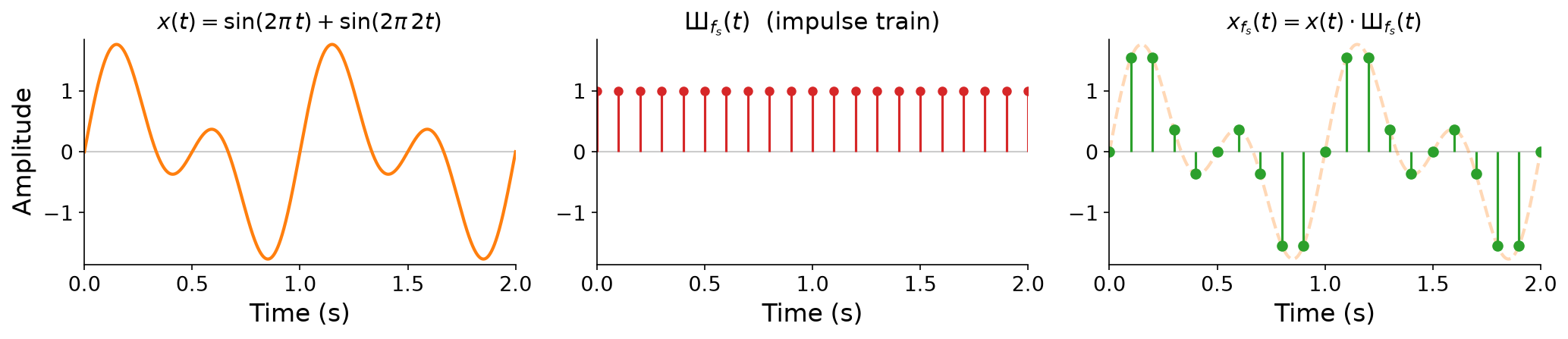
Fig. 31 Sampling as multiplication in the time domain. The running example \(x(t)\) (a sum of a 1 Hz and a 2 Hz sinusoid) is multiplied by the impulse train \(\text{Ш}_{f_s}(t)\) to give the sampled signal \(x_{f_s}(t) = x(t)\cdot\text{Ш}_{f_s}(t)\).

The frequency-domain view of sampling

Why bother reframing sampling as a multiplication? Because it lets us apply the Fourier transform. Recall from Chapter 5 that the Fourier transform associates any time-domain signal \(x(t)\) with a unique frequency-domain representation \(X(\omega)\). Crucially, the Fourier transform makes no assumption that \(x(t)\) is continuous or smooth. It only requires that the signal be defined across all of \(\mathbb{R}\). Our sampled signal \(x_{f_s}(t)\), spiky and discontinuous as it is, still has a perfectly well-defined frequency domain spectrum via the Fourier transform.

So what is the spectrum of the sampled signal? We’ll skip the calculus and show the result in the bottom row of the figure below. Multiplying by the impulse train in the time domain has the effect of copying the original spectrum \(X(\omega)\) around every integer multiple of the sampling rate \(f_s\). Where the original signal had frequency content only near zero, the sampled signal has infinitely many copies of that content, evenly spaced at \(0, \pm f_s, \pm 2f_s, \ldots\)

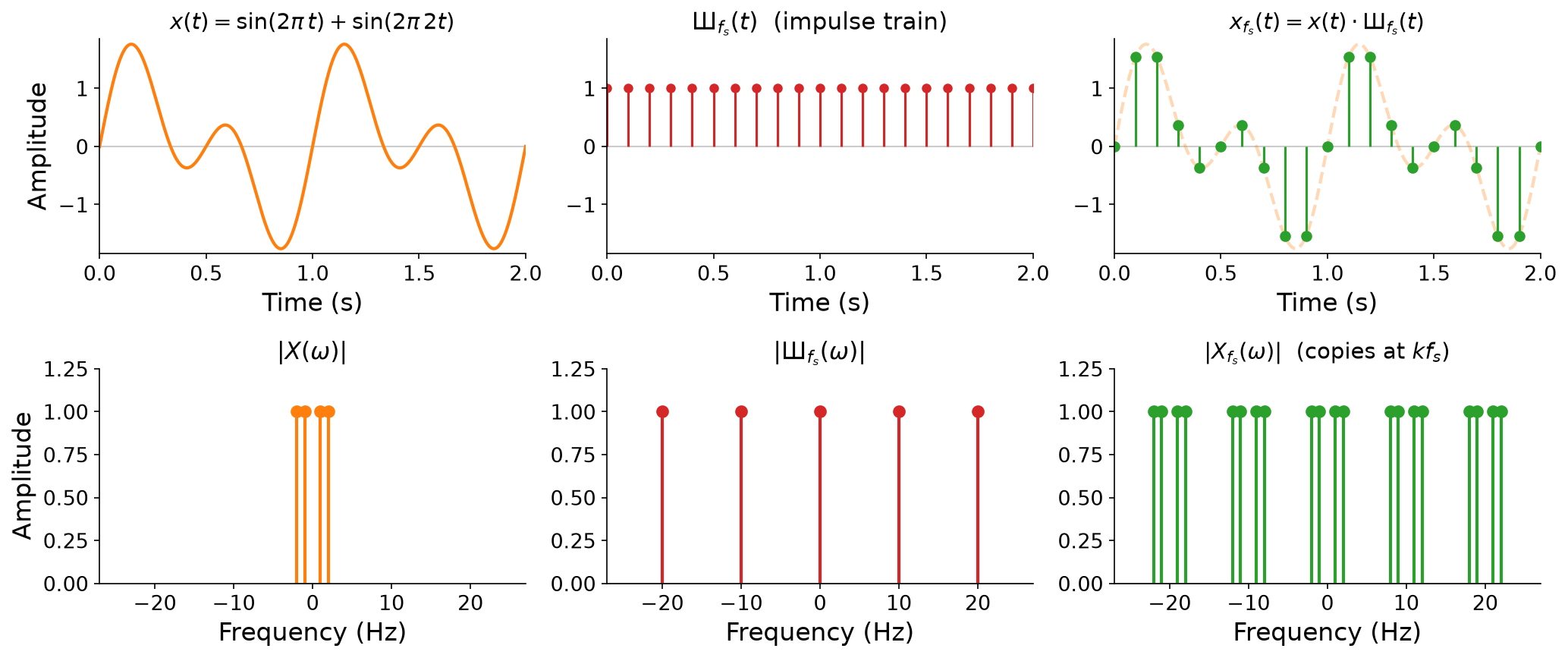
Fig. 32 Sampling as multiplication, viewed in both domains. Top (time): the running example \(x(t)\) times the impulse train \(\text{Ш}_{f_s}(t)\) gives the samples \(x_{f_s}(t)\). Bottom (frequency): the spectrum \(|X(\omega)|\) (spikes at \(\pm 1\) and \(\pm 2\) Hz) is replicated around every integer multiple of \(f_s\), producing \(|X_{f_s}(\omega)|\). (All spectral amplitudes are drawn at 1 for clarity.)

Definition 20 (Frequency-domain consequence of sampling)

Sampling a signal at rate \(f_s\) replicates its spectrum at every integer multiple of \(f_s\). If \(x(t)\) has spectrum \(X(\omega)\), then the sampled signal \(x_{f_s}(t)\) has spectrum

\[X_{f_s}(\omega) = \sum_{k=-\infty}^{\infty} X(\omega - k f_s).\]

Note

Why does multiplication in time produce copies in frequency? Multiplying two signals in the time domain corresponds to an operation called convolution in the frequency domain, and convolving a spectrum with a comb of spikes slides a copy of the spectrum to each spike. We will study convolution properly when we cover filtering in Chapter 9. For now, the key takeaway is just the result: sampling creates infinitely many copies of the spectrum, spaced \(f_s\) apart.

The widget below draws those copies for a signal whose bandwidth you control. Drag the sample rate down, or widen the band, and watch the neighbors close in on the original.

# hide
# no-output
from IPython.utils.capture import capture_output
with capture_output():
    %pip install -q plotly anywidget

import numpy as np
import plotly.graph_objects as go
from plotly.subplots import make_subplots
import ipywidgets as widgets
import icm_plotly
from icm_plotly import RED, BLUE, GOLD, IRON, TEAL, STEEL

Drag \(f_s\): the red baseband is the signal’s own spectrum, and the blue copies are the ones that sampling adds at every multiple of \(f_s\). The gold dashes mark \(\pm f_s / 2\). Lower \(f_s\), or widen the band with \(f_{\max}\), until the copies run into the baseband.

# hide
# autorun
FS0, FMAX0 = 1600.0, 500.0          # starting parameters

u = np.linspace(-1.0, 1.0, 181)     # one copy's shape, in units of f_max
S = (np.exp(-((np.abs(u) - 0.28) ** 2) / 0.018)
     + 0.55 * np.exp(-((np.abs(u) - 0.68) ** 2) / 0.010))
S *= 1.0 - np.abs(u) ** 8           # taper to zero at the band edges
S /= S.max()

KS = list(range(-4, 5))             # the copies we draw, centered at k * f_s
NK = len(KS)

def verdict(fs, fmax):
    return "clear" if fs > 2 * fmax else "touch" if fs == 2 * fmax else "overlap"

VERDICT = {"clear": "<b>copies clear</b>", "touch": "<b>copies touch</b>",
           "overlap": "<b>copies overlap</b>"}
VERDICT_COLOR = {"clear": IRON, "touch": GOLD, "overlap": RED}

def figure():
    fig = go.Figure()
    for k in KS:
        fig.add_scatter(x=k * FS0 + u * FMAX0, y=S, mode="lines",
                        line=dict(color=BLUE, width=1.3))
    fig.add_scatter(x=u * FMAX0, y=S, mode="lines",   # the baseband, on top
                    line=dict(color=RED, width=2.4))
    fig.add_scatter(x=[-FS0 / 2, -FS0 / 2, None, FS0 / 2, FS0 / 2, None],
                    y=[0, 1.12, None, 0, 1.12, None], mode="lines",
                    line=dict(color=GOLD, width=1.6, dash="dash"))
    state = verdict(FS0, FMAX0)
    fig.add_scatter(x=[2440], y=[1.16], mode="text", textposition="middle left",
                    text=[VERDICT[state]],
                    textfont=dict(size=17, color=VERDICT_COLOR[state]))
    fig.update_xaxes(range=[-2500, 2500], title_text="Frequency (Hz)",
                     fixedrange=True)
    fig.update_yaxes(range=[0, 1.26], title_text="Magnitude", fixedrange=True)
    return fig

def controls(fig):
    fs = widgets.FloatSlider(description="Sample rate $f_s$ (Hz)", min=400,
                             max=2400, value=FS0, step=50)
    fmax = widgets.FloatSlider(description=r"Band limit $f_{\max}$ (Hz)", min=100,
                               max=800, value=FMAX0, step=25)
    readout = widgets.HTML()

    # the defaults snapshot the arrays; the page's notebooks share one kernel
    def update(fs, fmax, u=u, KS=KS, NK=NK, verdict=verdict, VERDICT=VERDICT,
               VERDICT_COLOR=VERDICT_COLOR, readout=readout):
        state = verdict(fs, fmax)
        with fig.batch_update():
            for i, k in enumerate(KS):
                fig.data[i].x = k * fs + u * fmax
            fig.data[NK].x = u * fmax
            fig.data[NK + 1].x = [-fs / 2, -fs / 2, None, fs / 2, fs / 2, None]
            fig.data[NK + 2].text = [VERDICT[state]]
            fig.data[NK + 2].textfont.color = VERDICT_COLOR[state]
        relation = {"clear": "&gt;", "touch": "=", "overlap": "&lt;"}[state]
        readout.value = (f"<span style='font-size:0.9em'><i>f</i><sub>s</sub> = "
                         f"{fs:.0f} Hz &nbsp;{relation}&nbsp; 2<i>f</i><sub>max</sub> = "
                         f"{2 * fmax:.0f} Hz</span>")

    widgets.interactive_output(update, {"fs": fs, "fmax": fmax})
    return widgets.VBox([fs, fmax, readout])

icm_plotly.show(figure, controls)

Sample rate \(f_s\) (Hz)1600.00

Band limit \(f_{\max}\) (Hz)500.00

f_s = 1600 Hz  >  2f_max = 1000 Hz

What this means in practice

We can now view the whole analog-to-digital and digital-to-analog pipeline in terms of the frequency domain. Analog-to-digital conversion (ADC) takes a continuous sound \(x(t)\), multiplies it by an impulse train to produce samples \(x_{f_s}(t)\), whose spectrum \(X_{f_s}(\omega)\) consists of the infinite copies we just described:

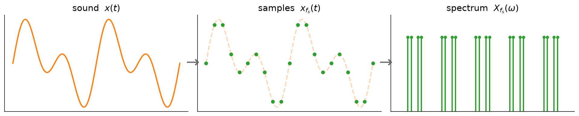
Fig. 33 Analog-to-digital conversion. The continuous sound \(x(t)\) is sampled into \(x_{f_s}(t)\), whose spectrum \(X_{f_s}(\omega)\) is the original spectrum replicated at every multiple of \(f_s\).

Digital-to-analog conversion (DAC) has to run this backwards. From the copied spectrum \(X_{f_s}(\omega)\), it must isolate the original spectrum \(X(\omega)\) (using a filter to discard the copies), and from that reconstruct the original sound \(x(t)\):

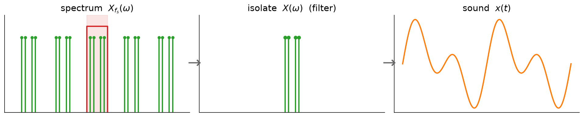
Fig. 34 Digital-to-analog conversion. A filter isolates the central copy \(X(\omega)\) from among the copies, discarding the rest, and the continuous sound \(x(t)\) is reconstructed from it.

This leads to the key insight at the heart of sampling:

Important

As long as we can perfectly identify and isolate the original spectrum \(X(\omega)\) among the shifted copies in \(X_{f_s}(\omega)\), we can perfectly reconstruct \(x(t)\) from the sampled version \(x_{f_s}(t)\).

This should feel surprising. Sampling is obviously throwing information away. It records the signal at a handful of instants and discards everything in between. In fact, infinitely many different continuous signals pass through the exact same samples. The figure below shows two sinusoids at 1 and 2 Hz that both cross zero at every integer, so sampled at \(f_s = 1\) Hz they yield identical (all-zero) samples:

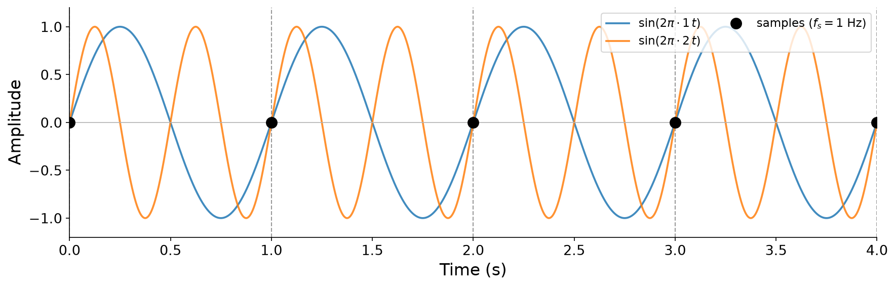
Fig. 35 Two different continuous signals that share identical samples. At \(f_s = 1\) Hz, both sinusoids are sampled at their zero crossings, so from the samples alone we cannot tell them apart.

Given that many signals share the same samples, it stands to reason that perfect reconstruction from samples can only work under the right conditions and assumptions. Understanding exactly when we can isolate the original spectrum is the heart of sampling theory.