import matplotlib
if not hasattr(matplotlib.RcParams, "_get"):
    matplotlib.RcParams._get = dict.get

9.1 Difference equations

In a digital signal processing context, a difference equation defines a filter by expressing each output sample as a formula in terms of the input samples. It is the most direct, hands-on way to specify a filter, and it translates immediately into code.

A first example

Consider the difference equation

\[\purple{y[n]} = \blue{x[n]} + \green{x[n-1]}.\]

Each output sample is the current input sample plus a delayed copy of the input. The term \(\green{x[n-1]}\) is the input shifted one sample later in time, in other words the value the input had one sample ago. Referring to a delayed copy of a signal like this, written \(\green{x[n-d]}\) for a delay of \(d\) samples, is the fundamental building block of every filter in this chapter, so make sure the idea feels natural before moving on.

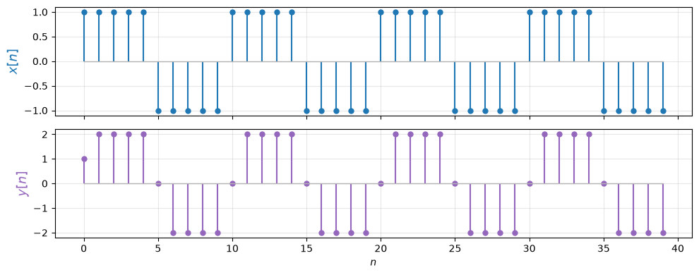
Let us feed the filter a simple square wave with a ten-sample period, \(x[n] = [1, 1, 1, 1, 1, -1, -1, -1, -1, -1, \ldots]\). To evaluate \(x[n-1]\) at the very start, we need \(x[-1]\), which lies before the signal begins. Throughout this chapter we adopt the standard convention that a signal is zero at any index outside its defined range: \(x[n] = 0\) for \(n < 0\). The very first output sample therefore sees a delayed copy that is still “warming up” from zero.

Fig. 49 The filter \(\purple{y[n]} = \blue{x[n]} + \green{x[n-1]}\) applied to a square wave. The delayed copy \(\green{x[n-1]}\) (green) is the input shifted right by one sample, with a zero assumed before \(n = 0\) (shaded). Summing it with \(\blue{x[n]}\) gives \(\purple{y[n]}\) (purple).

Comparing \(y[n]\) to \(x[n]\), a few things stand out:

1. The output has a larger peak amplitude, reaching \(\pm 2\) where the two copies agree.

2. It has a slightly different shape, with the square wave’s abrupt transitions softened into a step.

3. There is a brief “warm-up” at the very start.

Softening abrupt transitions is a hint that this filter smooths the signal by attenuating its high frequencies, which we will confirm later. You can experiment with this filter in code in the following example:

# hide
import numpy as np
import matplotlib.pyplot as plt
import pyquist as pq


def plot_filter_input_output(x, y):
    """Stem-plot an input (blue) above its filtered output (purple)."""
    fig, axes = plt.subplots(2, 1, figsize=(10, 4), sharex=True)
    for ax, data, label, color in zip(axes, [x, y], [r"$x[n]$", r"$y[n]$"], ["C0", "C4"]):
        ml, sl, bl = ax.stem(range(len(data)), data)
        plt.setp(ml, color=color, markersize=5)
        plt.setp(sl, color=color)
        plt.setp(bl, color="0.7", linewidth=1.0)
        ax.set_ylabel(label, color=color, fontsize=13)
        ax.grid(True, alpha=0.3)
    axes[-1].set_xlabel(r"$n$")
    plt.tight_layout()
    plt.show()

# The difference equation y[n] = x[n] + x[n-1], applied to a square wave.
# Edit the equation in the loop and re-run to explore other filters!
f_s = 44100
N = f_s                                       # one second of audio
n = np.arange(N)
x = np.where((n // 5) % 2 == 0, 1.0, -1.0)    # square wave, 10-sample period

y = np.zeros(N)
for n in range(N):
    if n - 1 < 0:                             # samples before the start are 0
        y[n] = x[n]
    else:
        y[n] = x[n] + x[n - 1]

# The same computation, vectorized:
# y = x + np.concatenate([np.zeros(1), x])[:N]

plot_filter_input_output(x[:40], y[:40])      # show the first 40 samples

A second example

Now consider a closely related difference equation that subtracts the delayed copy instead of adding it, and scales both terms by one half:

\[\purple{y[n]} = \tfrac{1}{2}\blue{x[n]} - \tfrac{1}{2}\green{x[n-1]}.\]

Fig. 50 The filter \(\purple{y[n]} = \tfrac{1}{2}\blue{x[n]} - \tfrac{1}{2}\green{x[n-1]}\) applied to the same square wave. Subtracting a delayed copy leaves the output zero wherever the input is constant and produces a spike only at each transition.

The behavior has both differences and similarities compared with the previous example:

1. The one-half factors keep the amplitude in check.

2. Subtracting a delayed copy makes the filter respond only to changes in the input, so the output is zero across the flat stretches and spikes at the transitions.

3. There is again a brief warm-up.

Responding only to change, and ignoring the steady stretches, is a hint that this filter discards low frequencies and keeps the high ones. This filter is, in effect, a crude edge detector.

What do these filters do to sound?

Difference equations are trivial to implement, but as the two examples show, their effect can be hard to predict just by reading the formula. The clearest way to build intuition is to listen. Below are the two filters applied to a burst of white noise, which contains every frequency in equal measure, so we can hear how each filter reshapes a full, flat spectrum:

Input white noise \(x[n]\)

\(y_1[n] = x[n] + x[n-1]\)

\(y_2[n] = \frac{1}{2}x[n] - \frac{1}{2}x[n-1]\)

By ear, the first filter sounds louder but potentially “darker” in frequency, while the second sounds “brighter”.

We can see this directly by plotting the amplitude spectrum of each filtered noise signal, alongside the flat spectrum of the input noise itself. Because the input is spectrally flat, each output spectrum traces out the filter’s own frequency response. The two filters are near-mirror images of each other:

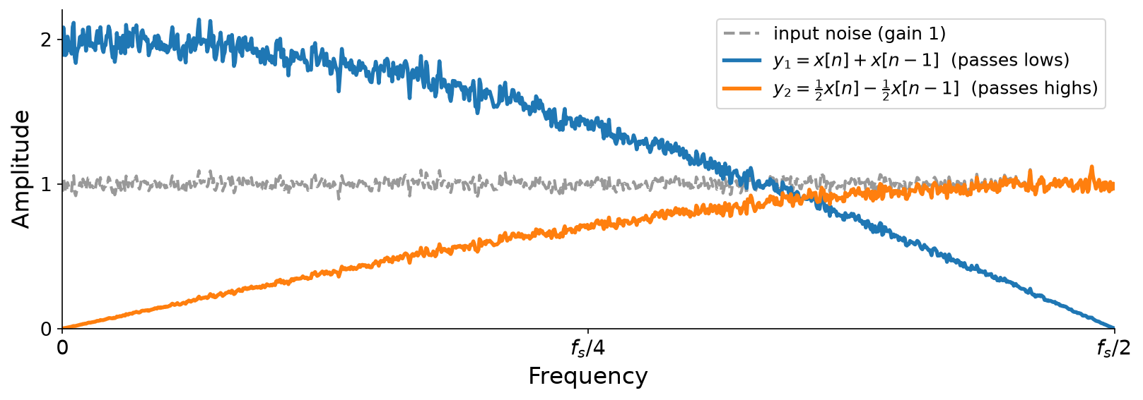
Fig. 51 The frequency response of each filter, measured by applying the filter to white noise and taking the DFT. Since the input noise is spectrally flat, each output spectrum reveals that filter’s frequency response.

The first, \(y_1\) (a sum of a signal and its delayed copy), passes the low frequencies through and rolls off the highs. Notice that at low frequencies its gain rises above \(1\), meaning it actually amplifies the input there, reaching a gain of \(2\).

The second, \(y_2\) (a difference), does the reverse, passing the high frequencies through. Note that \(y_2\)’s response tops out at exactly half the height of \(y_1\)’s, a direct consequence of its \(\tfrac{1}{2}\) coefficients.

So the sum passes the low frequencies through while the difference passes the high frequencies through. We reached both conclusions by ear and by eye, with no theory at all. Over the rest of the chapter we build up several more perspectives on filters like these, each revealing a different facet of how they work.