Template - Notebook

Template - Notebook#

This page is a living template for Jupyter notebook pages (.ipynb). It is a real notebook (content/templates/template-notebook.ipynb) that demonstrates features available only in notebooks — executable Pyquist code that runs at build time, the glue mechanism for weaving computed values into prose, and notebook cell tags for controlling display.

For prose-only syntax (text formatting, math, admonitions, figures, tables, exercises, cross-references, etc.) — which works in both .md and .ipynb files — see the Markdown Template.

Use it two ways:

As a reference — skim the rendered page to see what is available.
As a starting point — copy template-notebook.ipynb, rename it, and replace the cells with your own content.

1. Why author a page as a notebook?#

Every page in this book is one of two file types:

.md — a MyST Markdown file: Prose, math, and directives. Best for chapters that are mostly explanation. Code blocks are displayed but not executed. See the Markdown Template.
.ipynb — a Jupyter notebook (this page): Markdown cells and code cells. Code runs when the book is built, and its output — numbers, plots, audio players — is captured into the page. Best for anything that should demonstrate running code.

Markdown cells inside a notebook understand the same MyST syntax as a .md file, so a notebook is a strict superset. This template covers only the features unique to notebooks — see the Markdown Template for everything else.

Important

To make a page actually execute Pyquist code, author it as a notebook like this one.

2. Executable code: Pyquist#

Everything below runs when the book is built. Code cells execute top to bottom, and their output — text, plots, and audio players — is captured into the page. This is the whole reason to author a page as a notebook.

2.1 Synthesize a tone#

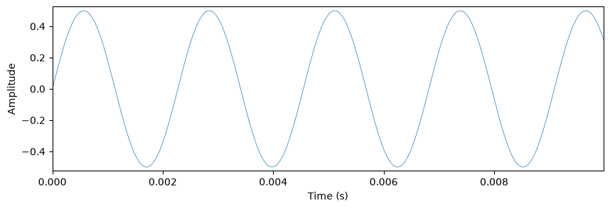
pq.Audio wraps a NumPy array of samples together with a sample_rate. Below is one second of a 440 Hz sine wave — concert A. pq.play renders an inline audio player you can click.

sr = 44100
t = np.arange(sr) / sr
tone = pq.Audio(0.5 * np.sin(2 * np.pi * 440 * t), sample_rate=sr)

print(f"shape={tone.shape}, sample_rate={tone.sample_rate} Hz, "
      f"duration={tone.duration:.2f} s, peak={tone.peak_amplitude:.2f}")

pq.play(tone)

shape=(44100, 1), sample_rate=44100 Hz, duration=1.00 s, peak=0.50

2.2 Visualize a signal#

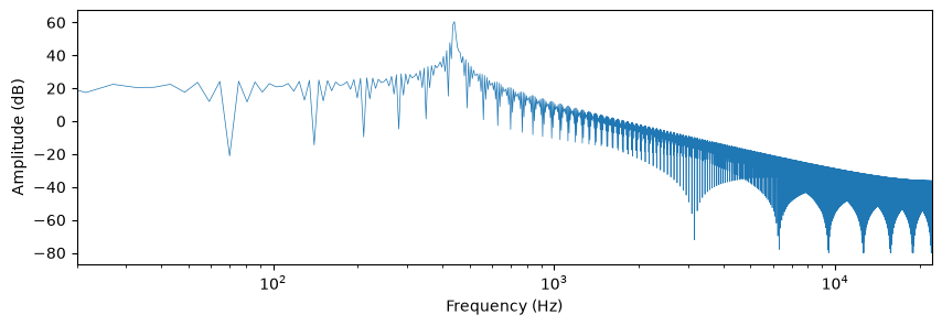
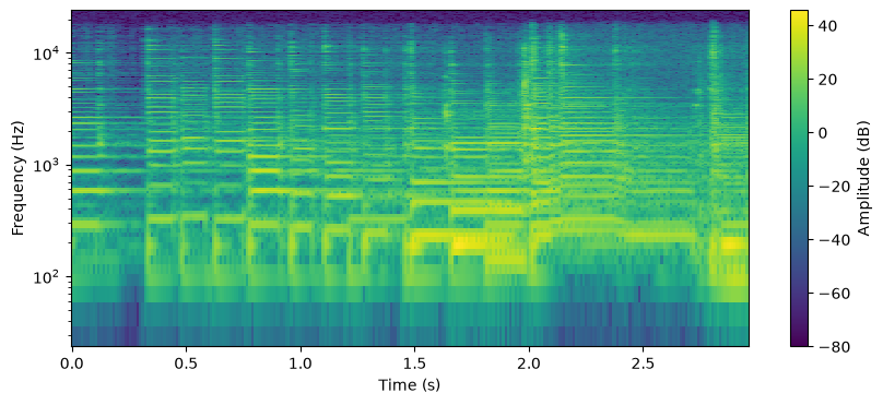
Pyquist ships three plotting helpers: plot (waveform), plot_freq (magnitude spectrum), and plot_spec (spectrogram). Each accepts offset / duration to zoom into a region.

pq.plot(tone, duration=0.01)       # first 10 ms of the waveform
pq.plot_freq(tone, duration=0.1)   # its frequency content

<Axes: xlabel='Frequency (Hz)', ylabel='Amplitude (dB)'>

../_images/a2b521a2dfa8b6285587b5d01d29a23617d7a2b8cd0cb89309bcac87028f99ec.png

../_images/24df7186d4ce265e44621cef0e4662aa5ca90ed3fcd0dc01c72bf76288ecea7d.png

2.3 Additive synthesis#

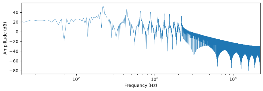
Summing harmonics builds a richer timbre. Here a sawtooth-like tone is built from ten harmonics with amplitudes \(A_k = 1/k\).

f0 = 220.0
saw = np.zeros_like(t)
for k in range(1, 11):
    saw += (1.0 / k) * np.sin(2 * np.pi * k * f0 * t)

saw_audio = pq.Audio(0.2 * saw, sample_rate=sr)
pq.plot_freq(saw_audio, duration=0.1)
pq.play(saw_audio)

../_images/9e7f36f95ccdf99a5af6a55c4b01ac1da2a3bfe937d55941b4da52e4f756c3a5.png

2.4 Load and transform audio#

Audio.from_file reads from disk (and Audio.from_url fetches from the web). Loaded audio can be sliced in time (segment), resampled (resample), and mixed to mono (as_mono) — each call returns a new Audio.

from pyquist.paths import TEST_DATA_DIR

riff = pq.Audio.from_file(
    TEST_DATA_DIR / "388954__fullmetaljedi__blues-riff-in-g-nylon.wav"
)
clip = riff.as_mono().segment(offset=0.0, duration=3.0)
print(f"{clip.duration:.2f} s at {clip.sample_rate} Hz")

pq.plot_spec(clip)
pq.play(clip)

3.00 s at 48000 Hz

../_images/c76c276635bc31d01d36e088dc8dad6470c9217286c9647f00d13cd9c999bf6b.png

2.5 Level, layout, and joining#

More Audio methods, each returning a new Audio (pass in_place=False to leave the original untouched): normalize sets a target peak in dBFS, clip hard-limits to [-1, 1], as_stereo / as_mono change the channel count, and Audio.concatenate joins clips end to end. (Audio.zeros(...) makes a silent buffer to fill in.)

# Each returns a new Audio.
quiet  = tone.normalize(peak_dbfs=-12.0, in_place=False)              # set peak level
safe   = tone.normalize(peak_dbfs=3.0, in_place=False).clip(in_place=False)  # hard-limit
stereo = tone.as_stereo()                                            # mono -> 2 channels
both   = pq.Audio.concatenate([tone, quiet])                         # join end to end

print(f"quiet peak={quiet.peak_amplitude:.3f}, clipped peak={safe.peak_amplitude:.3f}, "
      f"stereo channels={stereo.num_channels}, joined={both.duration:.1f}s")
pq.play(both)

quiet peak=0.251, clipped peak=1.000, stereo channels=2, joined=2.0s

2.6 Pitch and decibel helpers#

pyquist.helper converts between the units you reach for constantly: MIDI pitch ↔ frequency (pitch_to_frequency, frequency_to_pitch), note names → pitch (pitch_name_to_pitch), and decibels ↔ linear amplitude (db_to_amplitude, amplitude_to_db). All are vectorized over NumPy arrays.

from pyquist.helper import (
    pitch_to_frequency, frequency_to_pitch, pitch_name_to_pitch,
    db_to_amplitude, amplitude_to_db,
)

print(f"A4 (MIDI {pitch_name_to_pitch('A4')}) = {pitch_to_frequency(69):.1f} Hz")
print(f"440 Hz -> MIDI {frequency_to_pitch(440):.1f}")
print(f"-6 dB -> amplitude {db_to_amplitude(-6):.3f}, "
      f"amplitude 0.5 -> {amplitude_to_db(0.5):.1f} dB")

A4 (MIDI 69) = 440.0 Hz
440 Hz -> MIDI 69.0
-6 dB -> amplitude 0.501, amplitude 0.5 -> -6.0 dB

2.7 Scores and instruments#

A Score is a list of Events. An instrument is a function from an event to an Audio. score.render(instrument, metronome=...) turns the score into sound.

from pyquist.score import Score, Event, BasicMetronome
from pyquist.helper import pitch_to_frequency


# An instrument is called as instrument(**event.kwargs): it declares the
# kwargs it uses and absorbs the rest with **kwargs.
def pluck(pitch, duration, **kwargs):
    n = int(duration * sr)
    tt = np.arange(n) / sr
    freq = pitch_to_frequency(pitch)
    samples = 0.3 * np.sin(2 * np.pi * freq * tt) * np.exp(-4 * tt)
    return pq.Audio(samples, sample_rate=sr)


melody = Score([
    Event(0, {"pitch": 60, "duration": 0.5}),   # C
    Event(1, {"pitch": 64, "duration": 0.5}),   # E
    Event(2, {"pitch": 67, "duration": 0.5}),   # G
    Event(3, {"pitch": 72, "duration": 1.0}),   # C
])

pq.play(melody.render(pluck, metronome=BasicMetronome(bpm=120)))

2.8 MIDI files#

Score.from_midi parses a MIDI file into a (score, metronome) pair — each note becomes an Event carrying pitch, velocity, duration (seconds), program, and is_drum. The metronome converts between MIDI ticks and seconds, so you can segment a span and render it with an instrument.

from pyquist.paths import TEST_DATA_DIR

# A public-domain copy of Ravel's Boléro ships with pyquist.
score, metronome = pq.Score.from_midi(TEST_DATA_DIR / "ravel_bolero.mid")
print(f"{len(score)} notes, {metronome.tick_to_seconds(score.end_time):.0f}s long")


# Noise for drum events, the pluck from §2.7 for pitched ones.
def midi_instrument(is_drum, duration, **kwargs):
    if is_drum:
        n = int(duration * sr)
        env = np.exp(-30 * np.arange(n) / sr)
        return pq.Audio(0.1 * np.random.randn(n).astype(np.float32) * env, sample_rate=sr)
    return pluck(duration=duration, **kwargs)


# Render an 8-second excerpt; the metronome maps seconds to MIDI ticks.
excerpt = score.segment(
    offset=metronome.seconds_to_tick(11),
    duration=metronome.seconds_to_tick(8),
)
pq.play(excerpt.render(midi_instrument, metronome=metronome))

33249 notes, 958s long

2.9 Controlling cell display#

Notebook cell tags control what appears in the book. Add them to a cell’s metadata ("tags": [...]):

Tag	Effect
`hide-input`	Collapses the code; output stays visible.
`hide-output`	Collapses the output.
`remove-input`	Drops the code entirely; shows only output.
`remove-cell`	Drops the whole cell from the book.
`scroll-output`	Puts long output in a scrolling box.

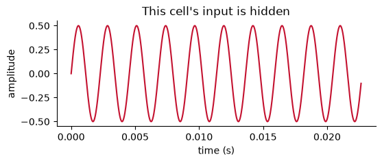
The next cell is tagged hide-input — you see its plot, but must click to reveal the code.

../_images/f7e7c2b4b270404d2c43dcd578243e893f0d7943030c5e5b87dfe7fabd7a7f59.png

3. Glue: weave computed values into prose#

The glue function (from MyST-NB) captures a value or figure in a code cell so it can be embedded later in any markdown cell — keeping prose and numbers in sync. The next code cell glues one number and one figure.

from myst_nb import glue

peak_db = 20 * np.log10(saw_audio.peak_amplitude)
glue("peak_db", round(float(peak_db), 1), display=False)

fig, ax = plt.subplots(figsize=(6, 2.4))
ax.magnitude_spectrum(saw_audio.as_mono().samples.ravel(), Fs=sr, scale="dB")
ax.set(xlim=(0, 3000), title="Sawtooth spectrum")
ax.spines[["top", "right"]].set_visible(False)
glue("spectrum_fig", fig, display=False)
plt.close(fig)

A glued value drops straight into a sentence: the sawtooth peaks at -9.3 dBFS. A glued figure is placed with the {glue:figure} directive:

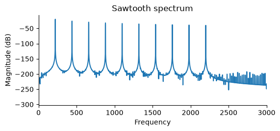
../_images/5a84d4beac5814ed2bf1fa3a48cc2b67dbfd89fc84e4251b6bc80019c8cbaeff.png — Fig. 75 A figure computed in a code cell and placed here with `{glue:figure}`.#

4. Record your own audio (live only)#

Run the cell below, click ● Record, allow microphone access, and speak — an inline player lets you hear your take. Then run the next cell to plot and play it.

In the browser, pq.record() automatically detects the Pyodide runtime and captures from the mic via the Web Audio API instead of a sound card — no flag needed. Because the capture is interactive, the returned Audio starts empty and fills in once you click Record, so read it in the next cell. These cells are tagged skip-execution: they run in your browser, not at build time.

# Click ● Record, allow the microphone, then speak for a few seconds.
clip = pq.record(3.0)

# `clip` fills in once you click Record above — then plot and play it.
print(f"recorded {clip.duration:.2f}s at {clip.sample_rate} Hz")
pq.plot(clip)
pq.play(clip)

5. Browser limits: what to expect when you click Run#

Code on this page runs in your browser (Pyodide / WebAssembly), where audio file support is limited to WAV. The cells below deliberately hit those limits so you can see the exact message each one raises. They are tagged skip-execution, so the built page shows no output — click ▶ Run on each to trigger it live. On your own computer, with the full libraries installed, every one of these works normally.

Cell	Operation	Expected live result
5.1	Read an MP3 (`Audio.from_file`)	`LibsndfileError` — WAV only
5.2	Write a non-WAV file (`Audio.write`)	`LibsndfileError` — WAV only

Reading WAV works fine in the browser (see §2.4). Recording and playback work too (see §4). Networking differs as well: Audio.from_url(...) relies on Python sockets the sandbox doesn’t provide, so it also fails here.

Installing packages (5.3) is the exception that works: !pip install <name> succeeds live for pure-Python packages, and for compiled ones bundled with this book (scipy, for example). Anything else raises an OSError saying so — as does any other ! shell command (!ls), because the browser has no shell.

# 5.1 — In the browser, only WAV audio can be read.
# (pyquist bundles this MP3, so it is already on the in-browser filesystem.)
from pyquist.paths import TEST_DATA_DIR

drums = pq.Audio.from_file(TEST_DATA_DIR / "434013__mrpearch__drum-patern.mp3")
pq.play(drums)

# 5.2 — Writing a non-WAV format errors instead of writing mislabeled data.
beep = pq.Audio(0.2 * np.sin(2 * np.pi * 440 * np.arange(8000) / 8000),
                sample_rate=8000)
beep.write("beep.mp3")

# 5.3 — Installing packages live: !pip install works for pure-Python wheels
# (compiled packages must be bundled with the book, like scipy).
!pip install pyjokes
import pyjokes

print(pyjokes.get_joke())

6. Using this template#

To start a new notebook chapter:

Copy content/templates/template-notebook.ipynb.
Rename it and move it into a chNN-*/ folder.
Register it in _toc.yml.
Replace these cells with your content.

Before publishing

Remove this Notebook Template page from _toc.yml — it is an author reference, not course content.

Note

Executable pages need Pyquist installed in the build environment and execute_notebooks set to auto (or force) in _config.yml. Both are already configured in this repository.