import matplotlib
if not hasattr(matplotlib.RcParams, "_get"):
    matplotlib.RcParams._get = dict.get

13.5 Waveshaping

Distortion is an effect that “degrades” a signal, intentionally, to give it more grit or warmth. It is a staple of rock music, where guitarists drive their amplifiers so hard that the signal distorts. We have actually seen distortion before: the clipping of Chapter 1, which forces every sample into \([-1, 1]\),

\[y[n] = \min\big(1, \max(-1, x[n])\big).\]

Recall from Chapter 9 that clipping is not linear. Distortion effects are almost always non-linear, because only non-linear filters can create new frequency content. An LTI filter can only boost or attenuate the frequencies already present in a sound.

A classic technique for distortion is waveshaping, which passes every sample of a signal through a fixed function:

Definition 40 (Waveshaping)

Given a transfer function \(f : \mathbb{R} \to [-1, 1]\), waveshaping maps an input signal \(x[n]\) to the output signal

\[y[n] = f(x[n]).\]

The choice of transfer function determines the character of the distortion. Hard clipping, \(f(x) = \min(1, \max(-1, x))\), has sharp corners, which produce harsh high harmonics that can alias. Soft clipping, for example \(f(x) = \tanh(g x)\) with a drive \(g\), rounds off the corners smoothly, which produces gentler harmonics:

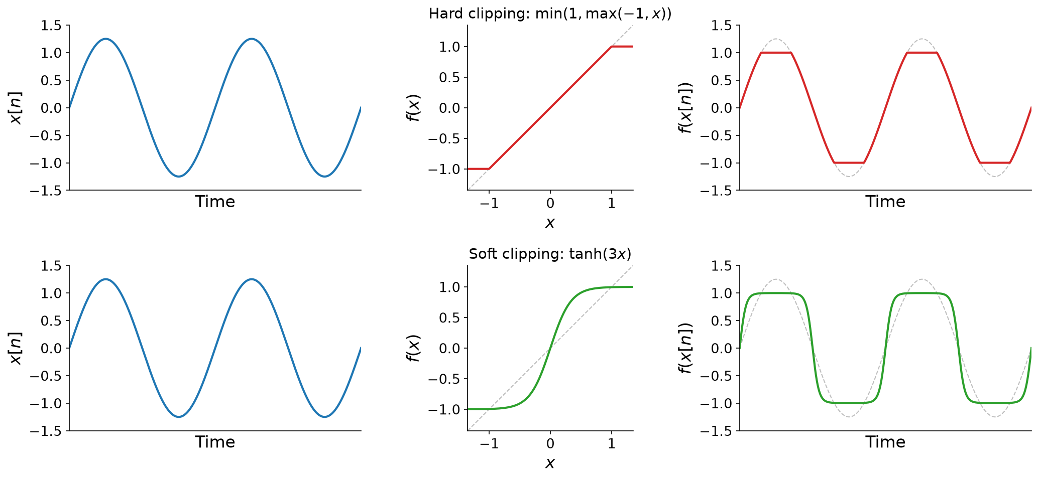
Fig. 104 Hard clipping (top) and soft clipping (bottom) of a sinusoid with an amplitude of \(1.25\) (left), via their transfer functions (middle), with the outputs on the right. Dashed lines show the identity \(f(x) = x\) and the input.

We can also design transfer functions that add specific harmonics, using the Chebyshev polynomials \(T_k\). Here are the first few:

\(k\)	\(T_k(x)\)
\(0\)	\(1\)
\(1\)	\(x\)
\(2\)	\(2x^2 - 1\)
\(3\)	\(4x^3 - 3x\)
\(4\)	\(8x^4 - 8x^2 + 1\)
\(5\)	\(16x^5 - 20x^3 + 5x\)

Each polynomial follows from the previous two by the recurrence \(T_{k+1}(x) = 2x \cdot T_k(x) - T_{k-1}(x)\) (see Wikipedia for more). The Chebyshev polynomials map \([-1, 1]\) onto \([-1, 1]\), and they satisfy \(T_k(\cos \theta) = \cos(k \theta)\). So waveshaping a full-scale sinusoid with \(T_k\) outputs exactly its \(k\)-th harmonic, and a weighted sum of Chebyshev polynomials outputs any desired mix of harmonics:

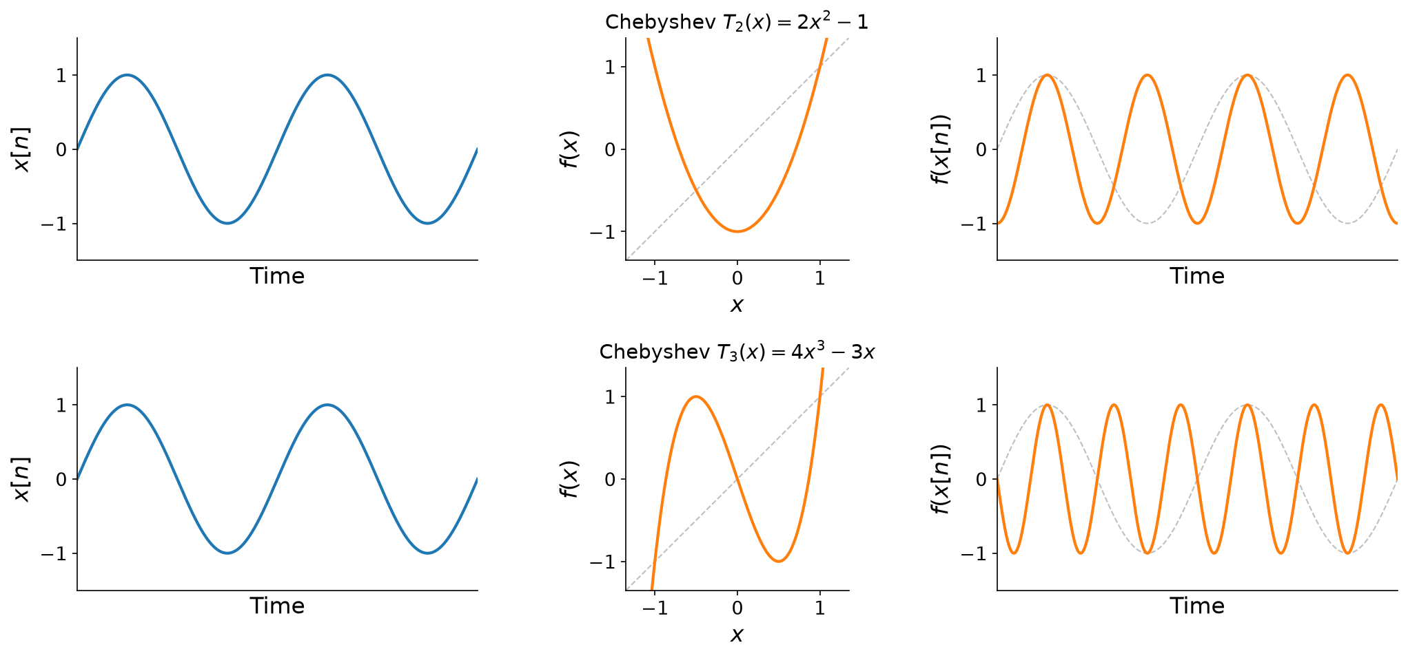
Fig. 105 Waveshaping a full-scale sinusoid (left) with the Chebyshev polynomials \(T_2\) and \(T_3\) (middle) doubles and triples its frequency (right).

Distortion

The code below distorts an acoustic guitar with three transfer functions: (1) hard clipping, (2) soft clipping, and (3) a wavefolder, \(f(x) = \sin(x)\), a favorite of modular synthesizers. Rather than flattening the peaks of a loud signal, a wavefolder folds them back toward zero, which creates a dense, metallic spectrum. Each transfer function is applied after amplifying the guitar by a drive of \(24\):

# hide
import numpy as np
import pyquist as pq
import matplotlib.pyplot as plt

def hard_clip(x: np.ndarray) -> np.ndarray:
    return np.clip(x, -1.0, 1.0)


def soft_clip(x: np.ndarray) -> np.ndarray:
    return np.tanh(x)


def wavefold(x: np.ndarray) -> np.ndarray:
    return np.sin(x)                          # folds back toward zero once |x| passes pi / 2


u = np.linspace(-6, 6, 1000)
for f in [hard_clip, soft_clip, wavefold]:
    plt.plot(u, f(u), label=f.__name__)
plt.xlabel("$x$")
plt.ylabel("$f(x)$")
plt.legend()
plt.show()

guitar = pq.Audio.from_file("./assets/guitar-acoustic.wav")
drive = 24.0                                   # push the guitar far into each nonlinearity
pq.play(guitar, normalize=True)
for f in [hard_clip, soft_clip, wavefold]:
    pq.play(pq.Audio(f(drive * guitar.samples[:, 0]), guitar.sample_rate), normalize=True)

Sound from Freesound: 187700 by afrodrumming, License: Attribution 4.0.

See also

Many distortion effects imitate analog hardware, like guitar amplifiers and their vacuum tubes. Simulating such circuits is the subject of virtual analog modeling. See Julius Smith’s overview of virtual analog synthesis and Kurt Werner’s dissertation on modeling audio circuits [Wer16].