12.0 Musical acoustics#
Recall from Chapter 1 that sound emerges when something in the world moves and disturbs the air around it, like a plucked guitar string. Musical instruments are carefully designed to vibrate in particular ways. In this section, we study the physics of these vibrations, which we will refer to as musical acoustics. We focus on musical acoustics of strings, which will be the basis of our physical model, and then briefly look at other kinds of instruments.
Waves in a medium#
A wave transfers energy from one point to another through a medium, like a string or the air. As a wave passes by, each particle of the medium is displaced temporarily, and then returns to its resting position. In other words, it is the disturbance that travels, not the medium itself. For example, when you flick one end of a long rope, a pulse travels along the rope. Each piece of the rope moves up and back down as the pulse passes by, but no piece of the rope travels along the direction of the pulse.
Three behaviors of waves are critical for musical acoustics:
Propagation. A wave travels through a medium at a speed \(v\), measured in \(\frac{\text{meters}}{\text{second}}\) (m/s), which depends on the properties of the medium. For example, sound travels through air at about \(343\) m/s, and waves travel along the strings of a guitar at roughly \(100\) to \(430\) m/s, depending on its tension.
Superposition. When two waves traveling in opposite directions meet, they pass through each other undisturbed. While they overlap, the displacement of the medium at each point is simply the sum of the displacements of the two waves. This principle, called superposition, is a physical example of the linearity that we studied in Chapter 9.
Reflection. When a wave reaches a rigid boundary, like the fixed end of a string, it reflects back with opposite polarity: a pulse that displaced the string upward returns displacing it downward. Intuitively, the boundary pushes back on the string with an equal and opposite force, as in Newton’s third law.
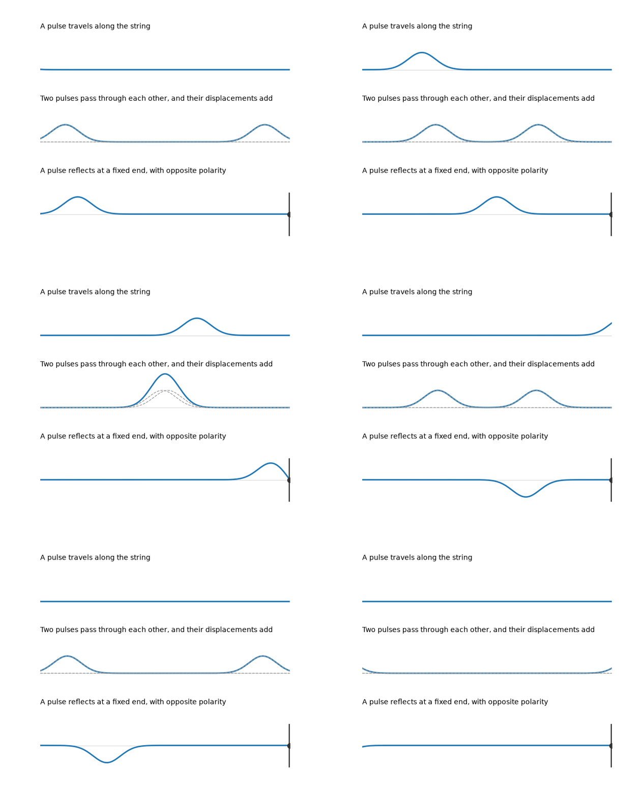
Fig. 79 Three behaviors of waves on a string: propagation (top), superposition (middle), and reflection (bottom). In the middle row, the dashed gray lines trace each pulse on its own, and the solid line is their sum.#
Standing waves#
When we pluck a string that is fixed at both ends, like on a guitar, waves travel in both directions along the string and reflect off its ends, again and again. At any moment, the string carries waves traveling both to the right and to the left, and by superposition, its shape is their sum. The result is a standing wave, which oscillates in place rather than traveling along the string. Some points on the string, called nodes, never move at all. Halfway between the nodes are the antinodes, where the string oscillates with the largest amplitude. The animation below shows two waves traveling in opposite directions, and the standing wave that they form:
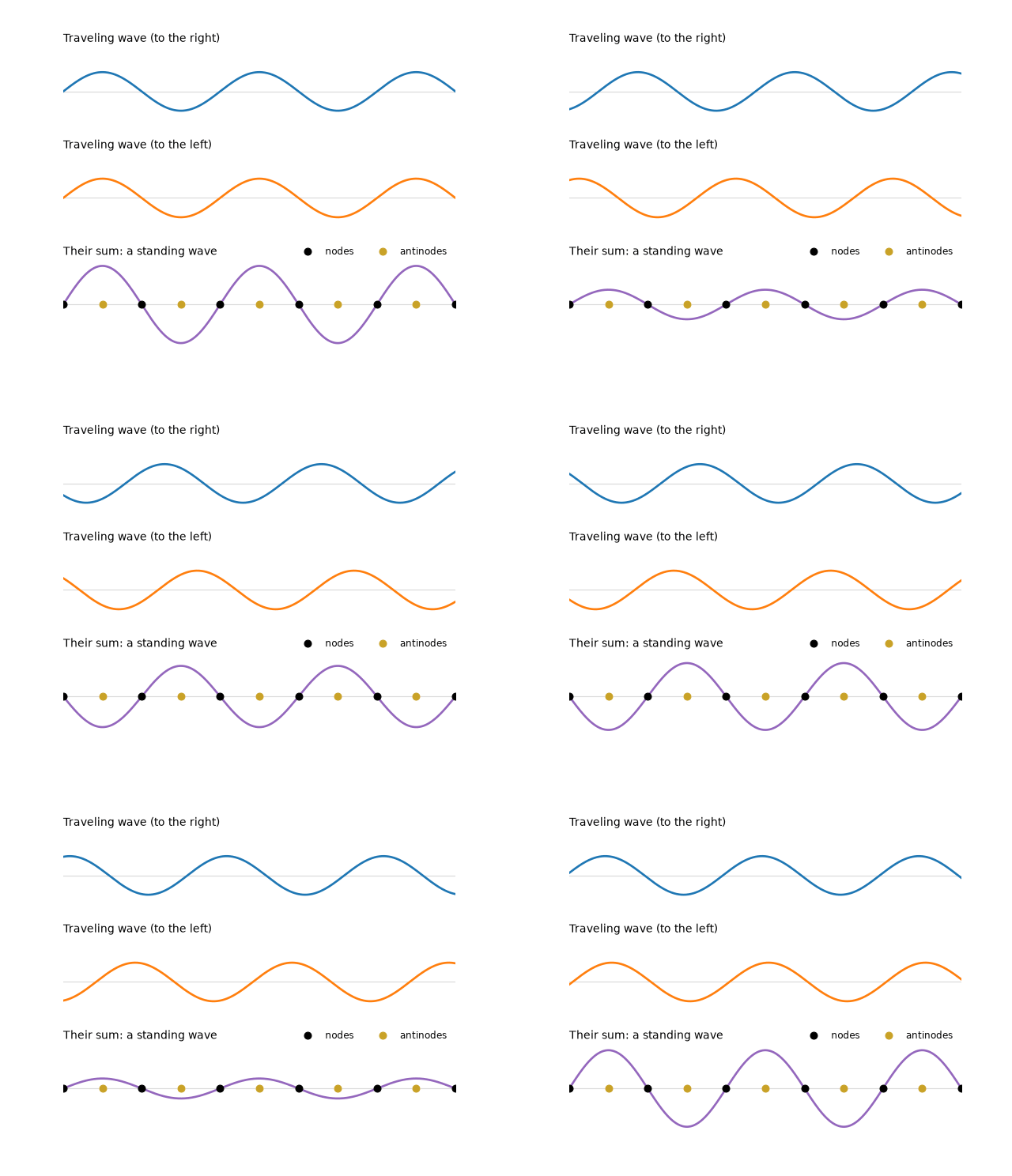
Fig. 80 Two sinusoids traveling in opposite directions (top and middle) sum to a standing wave (bottom). The nodes (black) never move, and the antinodes (gold) oscillate with the largest amplitude.#
Wavelength#
Where exactly are the nodes of a standing wave? To answer this, we need to describe how a wave varies in space, not just in time.
Suppose we shake one end of a long string up and down in a sinusoidal motion with frequency \(f\), sending a wave along the string at speed \(v\). Each point on the string then repeats the same sinusoidal motion, delayed by the time it takes the wave to reach it. So if we watch any one point over time, we see a sinusoid in time, like the signals we have studied throughout this book. But if we take a snapshot of the whole string at one instant, we see a sinusoid in space. The distance between neighboring peaks of this snapshot is the wavelength.
Definition 34 (Wavelength)
The wavelength \(\lambda\) of a sinusoidal wave is the distance that it travels during one cycle. For a wave with frequency \(f\) traveling at speed \(v\),
Mathematically, a sinusoidal wave traveling to the left has displacement \(\sin\!\big(2\pi(\tfrac{x}{\lambda} + f t)\big)\) at position \(x\) (in meters) and time \(t\) (in seconds). At any fixed position \(x\), this is a sinusoid in time with frequency \(f\). At any fixed time \(t\), it is a sinusoid in space with period \(\lambda\). As time passes, its peaks move to the left at a speed of \(\lambda \cdot f = v\). The same wave traveling to the right has displacement \(\sin\!\big(2\pi(\tfrac{x}{\lambda} - f t)\big)\). Using the identity \(\sin a + \sin b = 2 \sin\frac{a + b}{2} \cos\frac{a - b}{2}\), their sum is
Space and time have separated in the result. The sum is a fixed shape in space, \(\sin(2\pi x / \lambda)\), whose amplitude oscillates in time, \(\cos(2\pi f t)\), which is exactly why a standing wave stays in place. Its nodes are wherever \(\sin(2\pi x / \lambda) = 0\), which happens every half wavelength. And at any one position \(x_0\), the displacement of the string is simply a sinusoid in time with frequency \(f\), \(2 \sin(2\pi x_0 / \lambda) \cos(2\pi f t)\). Vibrations like these, passed through the body of an instrument into the air, are what we hear:
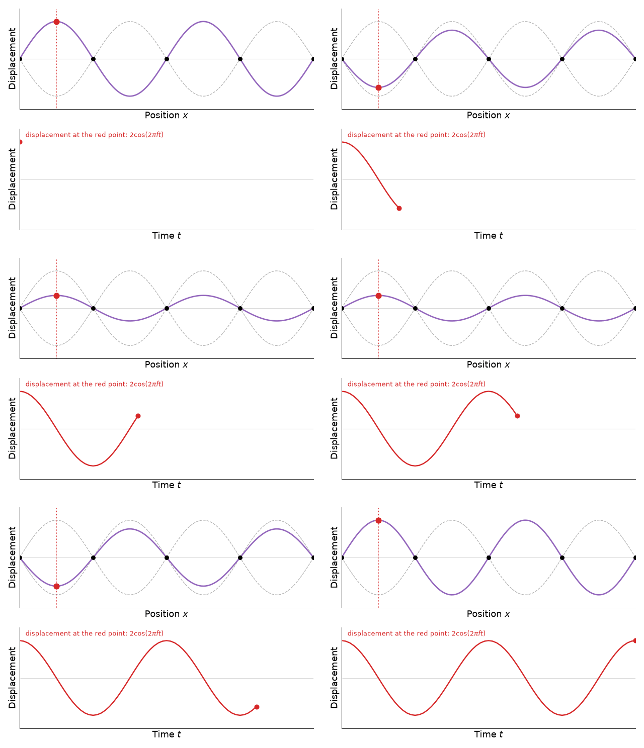
Fig. 81 A standing wave (top), and the displacement of one point on it over time (bottom). The red point is an antinode at \(x_0 = \frac{\lambda}{4}\), so its displacement traces out the sinusoid \(2 \cos(2\pi f t)\).#
Modes of oscillation#
Each standing wave that an object supports is called a mode of oscillation. Which modes does a string support? On a string of length \(L\) with both ends fixed, the ends cannot move, so they must be nodes. Since nodes occur every half wavelength, a standing wave fits on the string only if the string is a whole number of half wavelengths long:
Rearranging Definition 34, these modes have frequencies
So the lowest frequency is \(f_1 = \frac{v}{2L}\), and every other frequency is a whole-number multiple of it, \(f_i = i \cdot f_1\). These are exactly the harmonics of Chapter 3! A string fixed at both ends vibrates at a fundamental frequency \(f_1\) and its harmonics.
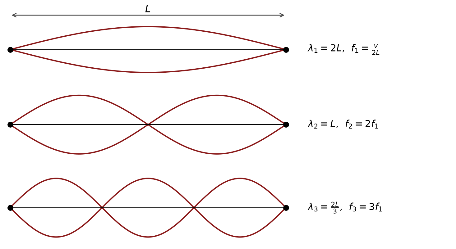
Fig. 82 The first three modes of a string of length \(L\) with both ends fixed. Each fits a whole number of half wavelengths between the ends.#
For example, the second-lowest string of a guitar vibrates along a length of about \(L = 0.65\) meters, and is tuned to a fundamental frequency of \(f_1 = 110\) Hz. So its longest wavelength is \(\lambda_1 = 2L = 1.3\) meters, and its waves travel at \(v = \lambda_1 \cdot f_1 = 1.3 \cdot 110 = 143\) m/s.
This also explains how to play different pitches on a string. A guitarist presses a string against a fret, which shortens the vibrating part of the string, decreasing \(L\) and raising \(f_1\). To change the frequency of a string without changing its length, we can instead change the speed \(v\), by changing the string’s tension or its material. Tightening a string raises its pitch, and thicker, heavier strings vibrate at lower pitches.
When we pluck a string, we excite many of its modes at once, and by superposition, its motion is their sum. So a plucked string produces a sum of sinusoids at harmonic frequencies, just like the Fourier series of Chapter 3. In previous chapters, we synthesized this sum directly. Now we see where it comes from.
The video below, from acoustician Daniel A. Russell, shows the motion of a plucked string. At first, its motion resembles a moving triangular pluck, which is the result of many modes vibrating at once. As the higher modes decay, it settles to resemble a standing wave at the fundamental.
Beyond strings#
Modes are not always equivalent to harmonics, though. Consider wind instruments, whose sound comes from a column of air vibrating inside a tube. At an open end of a tube, the air is free to move, so an open end is an antinode. At a closed end, the air cannot move, so a closed end is a node. A tube open at both ends, roughly like a flute, has antinodes at both ends, and the same wavelengths as a string, \(\lambda_i = \frac{2L}{i}\). But a tube closed at one end, roughly like a clarinet, has a node at one end and an antinode at the other. So its length must be an odd number of quarter wavelengths:
Its frequencies are \(f_i = (2i - 1) \cdot \frac{v}{4L}\): only the odd harmonics of a fundamental frequency \(\frac{v}{4L}\), which is an octave below that of an open tube of the same length.

Fig. 83 The first three modes of a string and of two kinds of tubes, labeled with their wavelengths \(\lambda\) and harmonic numbers \(h\). For the tubes, the curves show how far the air moves. The second and third modes of the closed tube are its third and fifth harmonics.#
In two dimensions, like a drumhead or a metal plate, modes become more intricate. Their frequencies are generally not whole-number multiples of the lowest one, which is part of why many percussion instruments have a less definite pitch than strings and winds. In the video below, also from Daniel A. Russell, particles sprinkled on a vibrating square plate collect along its nodal lines, where the plate stays still, revealing the shape of each mode. These shapes are called Chladni patterns, after Ernst Chladni, who studied them in the late 18th century.
Instruments vibrate in three dimensions, too. For example, the wooden body of a guitar has its own modes of oscillation, which help to amplify particular frequencies of the strings’ vibrations and radiate them into the air.
See also
To learn more about the acoustics of musical instruments, explore Daniel A. Russell’s acoustics and vibration animations, including the modes of drumheads and guitar bodies.