import matplotlib
if not hasattr(matplotlib.RcParams, "_get"):
    matplotlib.RcParams._get = dict.get

13.2 Tapped delay lines

So far, the delay \(M\) has been fixed. But we can also make the delay a function of time, \(M[n] > 0\):

\[y[n] = x[n] + g \cdot y[n - M[n]].\]

This requires a new mechanism, a tapped delay line. Before, a delay of \(M\) samples required a delay line of length \(M\), which we read at its far end. Now, we need a delay line long enough for the longest delay, \(M' = \max_n M[n]\), and we read it at a time-varying position in the middle, called a tap:

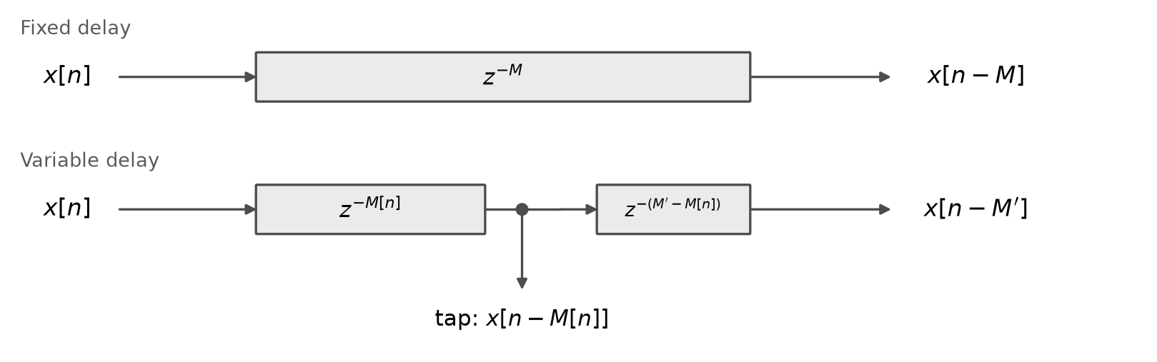
Fig. 96 A fixed delay line (top), and a delay line of length \(M'\) with a time-varying tap (bottom). The tap reads the delay line \(M[n]\) samples back from its input.

The delay line is still a circular buffer, and only the read position of the tap changes.

In addition to changing the amount of delay in a time-varying fashion, it would also be convenient to be able for thoes delay amounts to be fractional, rather than an integer number of samples. To achieve this, we can simply linearly interpolate between neighboring samples in our dealy line, just like the wavetables of Chapter 3.

The code below extends our feedback delay line to time-varying, fractional delays. To hear it in action, we sweep the delay of a comb filter from \(\frac{f_s}{110}\) samples down to \(\frac{f_s}{440}\) samples, while feeding it white noise. The pitch of the comb glides up two octaves:

# hide
import numpy as np
import pyquist as pq

def variable_feedback_delay(x: np.ndarray, M: np.ndarray, g: float = 1.0) -> np.ndarray:
    """A feedback delay line with a time-varying, fractional delay M[n] >= 1:
    y[n] = x[n] + g * y[n - M[n]]."""
    L = int(np.ceil(M.max())) + 2     # a delay line long enough for the longest delay
    buffer = np.zeros(L)
    i = 0                             # where y[n] will be written
    y = np.zeros(len(x))
    for n in range(len(x)):
        k = int(M[n])                 # whole samples of delay...
        a = M[n] - k                  # ...and the fraction left over
        # interpolate between y[n - k] and y[n - k - 1], like a wavetable (Chapter 3)
        delayed = (1 - a) * buffer[(i - k) % L] + a * buffer[(i - k - 1) % L]
        y[n] = x[n] + g * delayed
        buffer[i] = y[n]
        i = (i + 1) % L
    return y


f_s = 44100
noise = np.random.uniform(-1.0, 1.0, 3 * f_s)
M = np.linspace(f_s / 110, f_s / 440, len(noise))   # sweep the comb's teeth up two octaves
y = variable_feedback_delay(noise, M, g=0.95)
pq.play(pq.Audio(noise, f_s).normalize(peak_dbfs=-30.0))
pq.play(pq.Audio(y, f_s), normalize=True)

Flanging

Variable delays enable a classic effect called flanging. It originated with analog tape machines: engineers played the same recording on two tape machines at once, and slowed one down slightly by pressing a finger against the rim, or flange, of its tape reel. The small, varying delay between the two copies creates a comb filter whose teeth sweep up and down in frequency, which sounds like a whooshing jet plane.

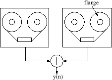
Fig. 97 Tape flanging: the same recording plays on two tape machines, whose outputs are summed. Pressing on the flange of a reel slows one machine down slightly, which delays its copy. Figure from Tamara Smyth’s course notes.

To simulate a flanger, we sweep the delay of a feedback delay line up and down with a slow sinusoid: around a center delay of \(M_c\) samples, by a relative depth \(A\) (between \(0\) and \(1\)), at a rate of \(f_m\) Hz:

\[M[n] = M_c \cdot \left(1 + A \sin\left(2\pi f_m \frac{n}{f_s}\right)\right).\]

Flangers typically use delays of just a few milliseconds. As the delay sweeps, so does the comb: its lowest tooth, at \(\frac{f_s}{M[n]}\), sweeps between a few hundred and a few thousand Hz. But while the delay sweeps sinusoidally, the comb does not. Its frequency is the reciprocal of the delay, so it lingers at low frequencies, and darts up to high frequencies whenever the delay is shortest:

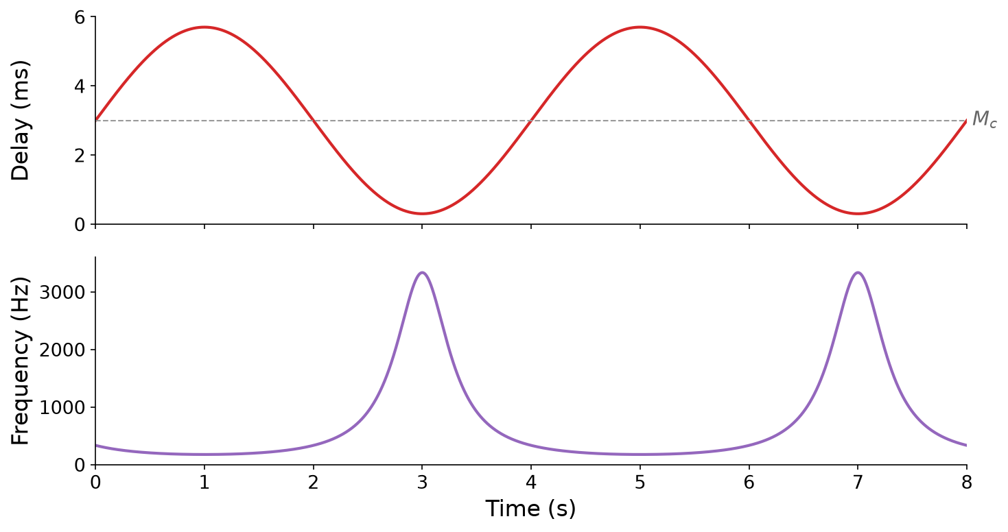
Fig. 98 The delay of a flanger with \(M_c = 3\) ms, \(A = 0.9\), and \(f_m = 0.25\) Hz (top), which sweeps between \(0.3\) and \(5.7\) ms every \(4\) seconds, and the corresponding frequency of the lowest tooth of its comb, \(\frac{f_s}{M[n]}\) (bottom), which sweeps between about \(175\) and \(3333\) Hz.

The code below applies this flanger to a synthesizer pad and to a distorted guitar:

# hide
import numpy as np
import pyquist as pq

# hide
def variable_feedback_delay(x: np.ndarray, M: np.ndarray, g: float = 1.0) -> np.ndarray:
    """A feedback delay line with a time-varying, fractional delay M[n] >= 1:
    y[n] = x[n] + g * y[n - M[n]]."""
    L = int(np.ceil(M.max())) + 2     # a delay line long enough for the longest delay
    buffer = np.zeros(L)
    i = 0                             # where y[n] will be written
    y = np.zeros(len(x))
    for n in range(len(x)):
        k = int(M[n])                 # whole samples of delay...
        a = M[n] - k                  # ...and the fraction left over
        # interpolate between y[n - k] and y[n - k - 1], like a wavetable (Chapter 3)
        delayed = (1 - a) * buffer[(i - k) % L] + a * buffer[(i - k - 1) % L]
        y[n] = x[n] + g * delayed
        buffer[i] = y[n]
        i = (i + 1) % L
    return y


def wet_ratio(db: float) -> float:
    """The wet ratio w that mixes the wet signal `db` decibels above the dry signal."""
    return 1 / (1 + pq.helper.db_to_amplitude(-db))

def flanger(x: np.ndarray, M_c: float, A: float, f_m: float, g: float,
            f_s: int) -> np.ndarray:
    """A feedback delay line whose delay sweeps around M_c samples:
    M[n] = M_c (1 + A sin(2 pi f_m n / f_s))."""
    n = np.arange(len(x))
    M = M_c * (1 + A * np.sin(2 * np.pi * f_m * n / f_s))
    return variable_feedback_delay(x, M, g)


pad = pq.Audio.from_file("./assets/pad.wav")
guitar = pq.Audio.from_file("./assets/guitar-distorted.wav")
w = wet_ratio(0.0)                            # equal parts wet and dry
for sound in [pad, guitar]:
    x = sound.samples[:, 0]
    f_s = sound.sample_rate
    wet = flanger(x, M_c=0.003 * f_s, A=0.9, f_m=0.25, g=0.7, f_s=f_s)   # around 3 ms, every 4 s
    pq.play(sound, normalize=True)
    pq.play(pq.Audio((1 - w) * x + w * wet, f_s), normalize=True)

Sounds from Freesound: pad 37746 by Quilt, License: CC0. Guitar 235538 by simosco, License: CC0.