12.2 Commuted synthesis#
The Karplus-Strong algorithm sounds remarkably like a plucked string, but it leaves us with a mystery. When we studied acoustics, we saw that a vibrating string carries two traveling waves, one moving right and one moving left, which superimpose to form standing waves. Karplus-Strong has only a single delay line, which doesn’t seem to correspond to any particular place on the string. So where are the traveling waves? In this section, we will answer this question at a high level, and along the way, learn a key trick (commuted synthesis) for making physical models efficient.
Digital waveguides#
A digital waveguide models the two traveling waves on a string explicitly, using two delay lines that run in opposite directions [SI92]. Each sample of delay corresponds to a particular point along the string. The upper delay line carries the right-going wave toward the bridge, and the lower one carries the left-going wave toward the nut. At each end, a wave reflects with opposite polarity, so the model multiplies it by \(-1\) and feeds it into the other delay line:
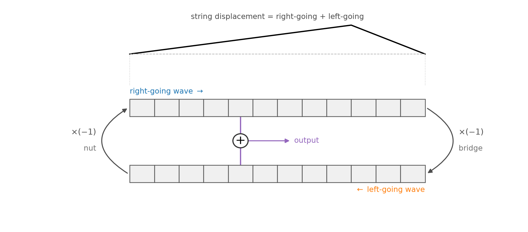
Fig. 92 A digital waveguide model of a string. Two delay lines carry the right-going and left-going waves, which invert as they reflect at each end. The displacement of the string at any point is the sum of the two waves at that point.#
This model has two key advantages:
It models the traveling waves explicitly. The structure of the simulation mirrors the physics of the string.
We can listen at any point along the string. By superposition, the displacement of the string at any point is simply the sum of the two delay lines at that point. For example, the pickups of an electric guitar sense the vibrations of its strings at particular points along their length, and the timbre depends on where the pickup is. Listening at the very middle of a string, we would hear none of its even harmonics, which all have nodes there.
Lumped losses#
So far, our waveguide is lossless, so its waves would travel back and forth forever. In a real string, energy is lost continuously, all along the length of the string. A faithful simulation would apply a tiny loss after every sample of delay, multiplying the wave by a gain \(g\) slightly less than \(1\). But this is computationally expensive: a string with a round trip of \(M\) samples would need \(M\) multiplications for every sample of output.
Fortunately, if we only listen at one point, we can lump these losses together into a single loss, and save almost all of that computation:
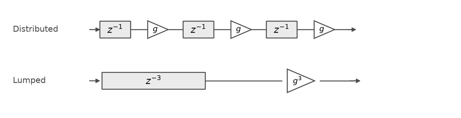
Fig. 93 Distributed losses (top) apply a loss \(g\) after every sample of delay, while lumped losses (bottom) apply them all at once, as \(g^3\). Both produce the same output, but the lumped version needs one multiplication instead of three.#
Why are these equivalent? Each delay and each loss is an LTI filter, i.e., a convolution with an impulse response. Recall from Chapter 9 that convolution is commutative and associative. So we can reorder and regroup a chain of filters however we like, without changing its output. Once we move all of the losses next to each other, the \(M\) losses of a round trip combine into a single gain, \(g^M\). The catch is that the signals in between the filters do change. So we can only lump losses together between the points where we listen.
This is the essence of commuted synthesis: a physical model is a chain of filters, and we can commute them into whatever order is cheapest to compute, even an order that makes no physical sense. The same idea applies to losses that depend on frequency. These are low-pass filters rather than gains, but they still lump together into a single low-pass filter.
Karplus-Strong, fully commuted#
We can now solve the mystery of the missing traveling waves. Consider a digital waveguide string with a round trip of \(M\) samples, so each delay line holds \(\frac{M}{2}\) samples. Suppose we only listen at the bridge, where a guitar string passes its vibrations to the body of the guitar. Then we can commute and lump everything else in the loop:
The two delay lines of \(\frac{M}{2}\) samples combine into a single delay line of \(M\) samples, one full round trip.
The two reflections, each multiplying by \(-1\), combine into a single multiplication by \((-1) \cdot (-1) = 1\), i.e., no inversion at all.
All of the losses along the way lump into a single loss. The \(M\) gains of \(g\) lump into \(g^M\), and the losses that depend on frequency lump into a single low-pass filter, like the two-point average of Karplus-Strong.
The result is exactly Karplus-Strong:
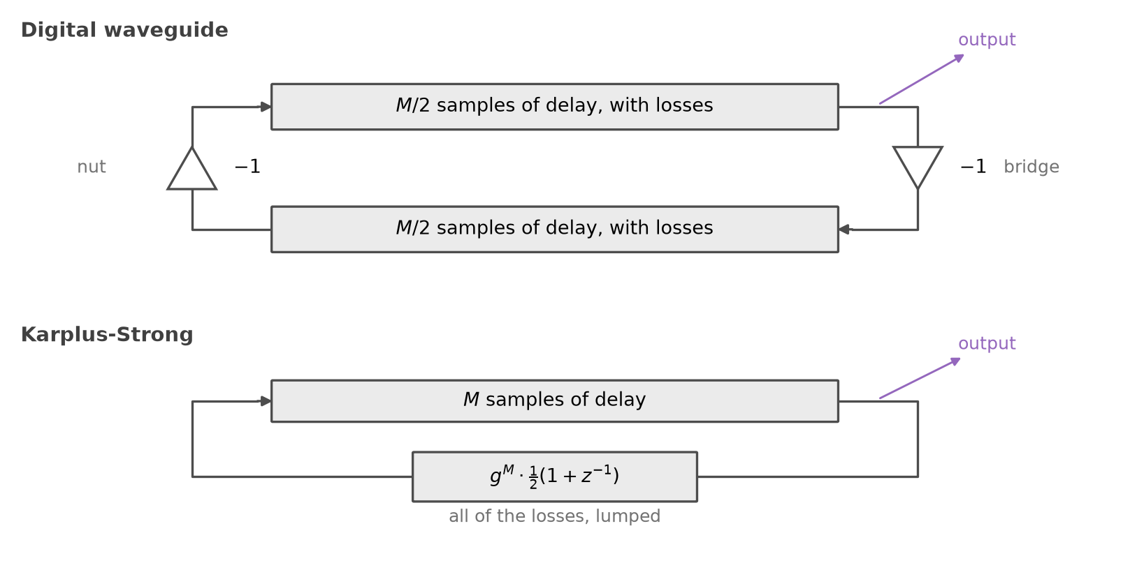
Fig. 94 Listening only at the bridge, a digital waveguide (top) commutes into Karplus-Strong (bottom). Adapted from a figure by Julius O. Smith III.#
In other words, Karplus-Strong is a fully commuted digital waveguide. The traveling waves are still there, but because we only listen at one point, we can commute them together into a single delay line. This makes Karplus-Strong extremely efficient, at the cost of the flexibility of the full waveguide.
Going further#
We have only scratched the surface of physical modeling. Researchers have spent decades refining these building blocks into models of nearly every kind of instrument, from bowed strings to brass, which are far more realistic than Karplus-Strong. Compared to the sample-based synthesis of Chapter 11, physical modeling has several advantages:
Complex sounds from simple laws: a few simple physical principles give rise to rich, intricate sounds.
Realistic transitions between notes: a physical model naturally simulates what happens between notes, like re-plucking a string that is still vibrating, while a sampler can only play back the transitions that were recorded.
Low memory usage: a physical model needs only a few parameters and some short delay lines, rather than gigabytes of recordings.
Modularity: building blocks can be recombined into new, hybrid instruments that could never be built in the physical world.
But it also has disadvantages:
Less realistic sound: even sophisticated physical models rarely sound as realistic as recordings of the real instrument.
Difficult control: like real instruments, physical models can be difficult to play. For example, producing a good sound from a model of a violin requires carefully controlling the pressure, speed, and position of the bow, just like a real violin.
Computational cost: simulating vibrations in two or three dimensions, like those of a drumhead or the body of a guitar, can be very expensive.
To dive deeper into the decades of research on physical modeling, see Julius Smith’s Physical Audio Signal Processing [SI10]. To experiment with sophisticated physical models in code, see the Synthesis ToolKit (STK), an open-source C++ library by Perry Cook and Gary Scavone, which includes physical models of flutes, clarinets, bowed strings, plucked strings, and more.