import matplotlib
if not hasattr(matplotlib.RcParams, "_get"):
    matplotlib.RcParams._get = dict.get

14.2 Linear predictive coding

So far, we have applied statistical models to scores. Can we also apply them to waveforms? Not directly, since \(n\)-gram models over individual audio samples aren’t particularly meaningful. With \(16\)-bit audio, the alphabet has \(2^{16} = 65{,}536\) states, so even a bigram model would have \(2^{32}\) probabilities, over four billion. And any tractable value of \(n\) would capture only microseconds of context. At \(f_s = 44{,}100\) Hz, a trigram model conditions on just two samples, about \(45\) microseconds of audio.

Instead of using \(n\)-grams to generate audio, we can use a similar approach to estimate filters. Consider a feedforward filter (Chapter 9) that aims to predict each sample of a signal \(x\) from the \(K\) samples before it:

\[\hat{x}[n] = h_1 \, x[n-1] + h_2 \, x[n-2] + \ldots + h_K \, x[n-K] = \sum_{k=1}^{K} h_k \, x[n-k].\]

Like an \(n\)-gram model, this filter uses a context of previous samples to predict the next one. But instead of a table of probabilities, it has just \(K\) coefficients, \(\mathbf{h} = [h_1, \ldots, h_K]\). How might we “learn” these coefficients from data?

Definition 47 (Linear predictive coding)

Given a signal \(\mathbf{x} \in \mathbb{R}^N\) and an order \(K\), linear predictive coding (LPC) finds the coefficients \(\mathbf{h} \in \mathbb{R}^K\) that minimize the total squared prediction error, \(e[n] = x[n] - \hat{x}[n]\):

\[\min_{\mathbf{h}} \sum_{n=K}^{N-1} e[n]^2 = \min_{\mathbf{h}} \sum_{n=K}^{N-1} \left(x[n] - \sum_{k=1}^{K} h_k \, x[n-k]\right)^2.\]

This is a basic statistical model. It predicts the current sample as a linear combination of the previous \(K\) samples, with coefficients that are fit to the statistics of the signal. Minimizing a sum of squared errors like this one is a classic problem called least squares. To set it up, we stack the context of each sample into a row of a matrix \(\mathbf{X} \in \mathbb{R}^{(N - K) \times K}\). Then the predictions for all of the samples at once are the matrix-vector product \(\mathbf{X} \mathbf{h}\):

\[\begin{split} \begin{bmatrix} \hat{x}[K] \\ \hat{x}[K+1] \\ \vdots \\ \hat{x}[N-1] \end{bmatrix} = \underbrace{\begin{bmatrix} x[K-1] & x[K-2] & \ldots & x[0] \\ x[K] & x[K-1] & \ldots & x[1] \\ \vdots & \vdots & \ddots & \vdots \\ x[N-2] & x[N-3] & \ldots & x[N-K-1] \end{bmatrix}}_{\mathbf{X}} \begin{bmatrix} h_1 \\ h_2 \\ \vdots \\ h_K \end{bmatrix}. \end{split}\]

For readers comfortable with linear algebra, least squares has a closed-form solution, \(\mathbf{h} = (\mathbf{X}^\top \mathbf{X})^{-1} \mathbf{X}^\top \mathbf{y}\), where \(\mathbf{y} = [x[K], \ldots, x[N-1]]\). In practice, solvers like np.linalg.lstsq compute it in more numerically stable ways.

Numerical libraries have efficient solvers for least squares. For example, NumPy’s np.linalg.lstsq finds the \(\mathbf{h}\) that minimizes the squared difference between \(\mathbf{X}\mathbf{h}\) and the true samples, \(x[K], \ldots, x[N-1]\). The code below fits an LPC model with \(K = 40\) to half a second of a sung vowel, and compares its predictions to the true samples. They are nearly indistinguishable:

# hide
import numpy as np
import matplotlib.pyplot as plt
import pyquist as pq

def lpc(x: np.ndarray, K: int) -> np.ndarray:
    """The coefficients h_1, ..., h_K that best predict each x[n] from x[n-1], ..., x[n-K]."""
    N = len(x)
    X = np.stack([x[K - k:N - k] for k in range(1, K + 1)], axis=1)   # row n: x[n-1], ..., x[n-K]
    h, *_ = np.linalg.lstsq(X, x[K:], rcond=None)                     # minimize the squared error
    return h


vowel = pq.Audio.from_file("./assets/vowel-a.wav")
f_s = vowel.sample_rate
x = vowel.segment(offset=1.0, duration=0.5).samples[:, 0].astype(np.float64)
K = 40
h = lpc(x, K)

# Predict every sample from the K samples before it
X = np.stack([x[K - k:len(x) - k] for k in range(1, K + 1)], axis=1)
prediction = X @ h
error = x[K:] - prediction
print(f"The prediction error is {10 * np.log10(np.sum(x[K:] ** 2) / np.sum(error ** 2)):.1f} dB "
      "quieter than the vowel")

t = 1000 * np.arange(K, K + 1000) / f_s
plt.figure(figsize=(10, 3.5))
plt.plot(t, x[K:K + 1000], label="$x[n]$")
plt.plot(t, prediction[:1000], "--", label=r"$\hat{x}[n]$")
plt.xlabel("Time (ms)")
plt.ylabel("Amplitude")
plt.legend(loc="upper right")
plt.show()
pq.play(vowel)

The prediction error is 41.7 dB quieter than the vowel

Recording from Freesound: 368728 by antoinevg, License: CC0.

Inverse filtering

What can we do with an LPC model? Let’s rearrange the definition of its prediction error:

\[e[n] = x[n] - \hat{x}[n] \quad \Longrightarrow \quad x[n] = e[n] + \hat{x}[n] = e[n] + h_1 \, x[n-1] + \ldots + h_K \, x[n-K].\]

This is a recursive filter (Chapter 9), whose input is the prediction error \(e\), and whose output is the original signal \(x\)! So LPC splits a signal into two parts: (1) a filter, described by just \(K\) coefficients, and (2) the prediction error, which is whatever the filter could not predict. A feedforward filter with the coefficients \([1, -h_1, \ldots, -h_K]\) turns \(x\) into \(e\), and a recursive filter with the same coefficients turns \(e\) back into \(x\). The two filters are inverses of each other. The code below confirms that this inverse filtering recovers the original signal, up to tiny rounding errors, for a recording of the vowel “E”:

# hide
import numpy as np
import matplotlib.pyplot as plt
import pyquist as pq
from scipy.signal import lfilter

# hide
def lpc(x: np.ndarray, K: int) -> np.ndarray:
    """The coefficients h_1, ..., h_K that best predict each x[n] from x[n-1], ..., x[n-K]."""
    N = len(x)
    X = np.stack([x[K - k:N - k] for k in range(1, K + 1)], axis=1)   # row n: x[n-1], ..., x[n-K]
    h, *_ = np.linalg.lstsq(X, x[K:], rcond=None)                     # minimize the squared error
    return h

vowel = pq.Audio.from_file("./assets/vowel-e.wav")
f_s = vowel.sample_rate
x = vowel.samples[:, 0].astype(np.float64)
h = lpc(vowel.segment(offset=1.0, duration=0.5).samples[:, 0].astype(np.float64), K=40)

# SciPy's lfilter(b, a, x) computes y[n] = sum_k b[k] x[n-k] - sum_{k>0} a[k] y[n-k]
coefficients = np.concatenate([[1.0], -h])     # [1, -h_1, ..., -h_K]
e = lfilter(coefficients, [1.0], x)             # e[n] = x[n] - sum_k h_k x[n-k]
y = lfilter([1.0], coefficients, e)             # y[n] = e[n] + sum_k h_k y[n-k]
print(f"Largest difference between x and y: {np.max(np.abs(x - y)):.1e}")

# Zoom in on 30 ms, with a dashed line every fundamental period (1 / 110 s)
start, length = f_s, int(0.03 * f_s)
t = 1000 * np.arange(length) / f_s
period = f_s / 110
first = np.argmax(np.abs(e[start:start + int(period)]))
fig, axes = plt.subplots(2, 1, figsize=(10, 5), sharex=True)
axes[0].plot(t, x[start:start + length])
axes[0].set_ylabel("$x[n]$")
axes[1].plot(t, e[start:start + length], color="C3")
axes[1].set_ylabel("$e[n]$")
axes[1].set_xlabel("Time (ms)")
axes[1].set_xlim(0, 30)
for k in range(4):
    for ax in axes:
        ax.axvline(1000 * (first + k * period) / f_s, color="0.6", ls="--", lw=1)
plt.show()
pq.play(pq.Audio(e, f_s), normalize=True)

Largest difference between x and y: 1.1e-12

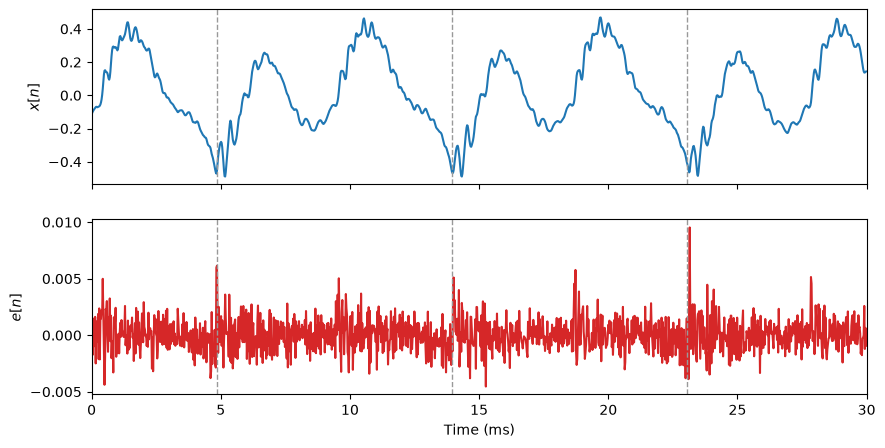
Notice that the prediction error is much quieter than the vowel. It is mostly noise, punctuated by a burst once every \(9\) ms or so (the dashed lines), which is exactly the period of the vowel. To see why, let’s take a closer look at the voice.

Recording from Freesound: 368727 by antoinevg, License: CC0.

Modeling vowels

The human voice is a natural fit for LPC. When we sing a vowel, our vocal folds vibrate, releasing a periodic series of puffs of air, called the glottal pulse train. The rate of the pulses is the fundamental frequency \(f_0\) of our voice, which sets its pitch, and the time between consecutive pulses is its fundamental period, \(t_0 = \frac{1}{f_0}\). For the recordings in this section, \(f_0 = 110\) Hz, so a pulse arrives every \(t_0 = \frac{1}{110} \approx 9.1\) ms.

Our throat and mouth then act as a filter, whose resonances, called formants, depend on the shape of our mouth. The formants determine which vowel we hear. This is known as the source-filter model of the voice.

LPC estimates this filter from a recording. Its prediction error contains whatever the filter cannot predict, which is approximately the glottal pulse train, a sharp pulse once per period. Each vowel gets a different filter, with formants at different frequencies:

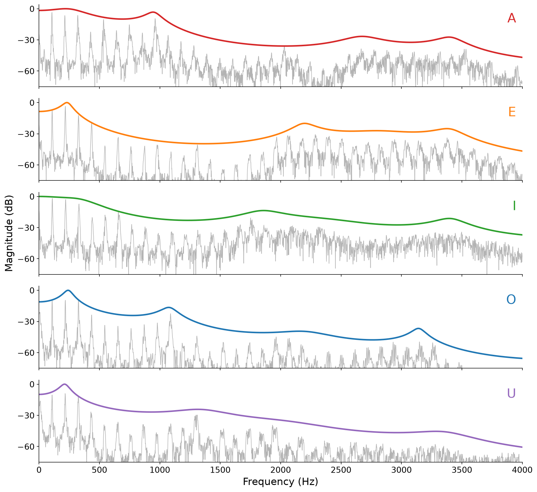
Fig. 117 The spectra of five vowels sung at \(110\) Hz (gray), and the frequency responses of their LPC filters, with \(K = 40\) (color). Each filter traces the envelope of its vowel’s harmonics. The peaks of the envelopes, the formants, differ from vowel to vowel.

So to synthesize a vowel, we can replace the prediction error with a synthetic train of impulses, and pass it through the LPC filter. The pulse train sets the pitch, and the filter sets the vowel, so we can change one without changing the other. The code below fits an LPC filter to each of the five vowels, and uses them to sing the first phrase of Twinkle, Twinkle, Little Star, changing vowels from note to note (A A E E I O U). Each note is a pulse train at the pitch of the note, faded in and out, and passed through the filter of its vowel:

# hide
import numpy as np
import pyquist as pq
from scipy.signal import lfilter

# hide
def lpc(x: np.ndarray, K: int) -> np.ndarray:
    """The coefficients h_1, ..., h_K that best predict each x[n] from x[n-1], ..., x[n-K]."""
    N = len(x)
    X = np.stack([x[K - k:N - k] for k in range(1, K + 1)], axis=1)   # row n: x[n-1], ..., x[n-K]
    h, *_ = np.linalg.lstsq(X, x[K:], rcond=None)                     # minimize the squared error
    return h

def pulse_train(f0: float, duration: float, f_s: int) -> np.ndarray:
    """A train of unit impulses, f0 of them per second: a crude glottal pulse train."""
    e = np.zeros(int(duration * f_s))
    e[::round(f_s / f0)] = 1.0
    return e


# An LPC filter for each vowel
paths = {"A": "./assets/vowel-a.wav", "E": "./assets/vowel-e.wav", "I": "./assets/vowel-i.wav",
         "O": "./assets/vowel-o.wav", "U": "./assets/vowel-u.wav"}
filters = {}
for name, path in paths.items():
    vowel = pq.Audio.from_file(path)
    x = vowel.segment(offset=1.0, duration=0.5).samples[:, 0].astype(np.float64)
    filters[name] = np.concatenate([[1.0], -lpc(x, K=40)])
f_s = vowel.sample_rate


def sing(pitch: int, vowel: str, duration: float, f_s: int) -> np.ndarray:
    """One note: a pulse train at the pitch, faded in and out, through the vowel's filter."""
    e = pulse_train(pq.helper.pitch_to_frequency(pitch), duration, f_s)
    n = np.arange(len(e))
    envelope = np.minimum(1.0, np.minimum(n / (0.02 * f_s), (len(e) - n) / (0.1 * f_s)))
    return lfilter([1.0], filters[vowel], envelope * e)


# Sing the first phrase of Twinkle, Twinkle, Little Star, changing vowels as we go
melody = [48, 48, 55, 55, 57, 57, 55]
vowels = "AAEEIOU"
durations = [0.5, 0.5, 0.5, 0.5, 0.5, 0.5, 1.0]
y = np.concatenate([sing(pitch, vowel, duration, f_s)
                    for pitch, vowel, duration in zip(melody, vowels, durations)])
pq.play(pq.Audio(y, f_s), normalize=True)

LPC was developed in the late 1960s and 1970s for compressing speech [Mak75]. Since the filter changes slowly, transmitting a few coefficients per frame takes far fewer bits than transmitting every sample. We will study audio compression in Chapter 16.

Recordings from Freesound by antoinevg, License: CC0: A 368728, E 368727, I 368726, O 368725, and U 368729.