6.1 Sidebands

import matplotlib
if not hasattr(matplotlib.RcParams, "_get"):
    matplotlib.RcParams._get = dict.get

6.1 Sidebands#

Here is a fixed carrier at 240 Hz ring-modulated by a modulator whose frequency climbs from 3 Hz to 48 Hz:

Modulator 3 Hz

Modulator 6 Hz

Modulator 12 Hz

Modulator 24 Hz

Modulator 48 Hz

A fixed 240 Hz carrier, ring-modulated at increasing rates.

An interesting perceptual shift emerges. At 3 Hz we clearly hear a single tone with fast tremolo. But by 48 Hz, we no longer hear tremolo at all. Instead we hear two distinct tones. Why does modulating a single frequency produce what sounds like multiple frequencies?

The answer is that ring modulation has a striking effect in the frequency domain. From two “input” sinusoids at frequencies \(\red{\omega_c}\) and \(\blue{\omega_m}\), it produces two completely different “output” sinusoids, at the sum and difference frequencies \(\purple{\omega_c + \omega_m}\) and \(\purple{\omega_c - \omega_m}\). The original input frequencies vanish from the spectrum entirely. These new frequencies are called sidebands, a general term for the frequency content that modulation creates on either side of a carrier. We will see sidebands emerge from every modulation technique in this chapter.

This behavior follows directly from a trigonometric identity. Recall the angle-sum and angle-difference identities for cosine:

\[\begin{split} \begin{aligned} \cos(A + B) &= \cos A \cos B - \sin A \sin B, \\ \cos(A - B) &= \cos A \cos B + \sin A \sin B. \end{aligned} \end{split}\]

Subtracting the first from the second cancels the cosine terms and leaves \(\cos(A - B) - \cos(A + B) = 2 \sin A \sin B\). Rearranging gives a product-to-sum identity that turns a product of sines into a sum:

\[\sin A \sin B = \tfrac{1}{2}\big[\cos(A - B) - \cos(A + B)\big].\]

Substituting \(A = \red{\omega_c} t\) and \(B = \blue{\omega_m} t\), we can rewrite ring modulation as a sum of two sinusoids:

\[\sin(\red{\omega_c} t)\,\sin(\blue{\omega_m} t) = \tfrac{1}{2}\cos\big((\purple{\omega_c - \omega_m})\,t\big) - \tfrac{1}{2}\cos\big((\purple{\omega_c + \omega_m})\,t\big).\]

There they are: two sinusoids, at \(\purple{\omega_c - \omega_m}\) and \(\purple{\omega_c + \omega_m}\), each with amplitude \(\tfrac{1}{2}\), and a phase shift from \(\sin\) to \(\cos\). The carrier and modulator frequencies themselves are nowhere to be found.
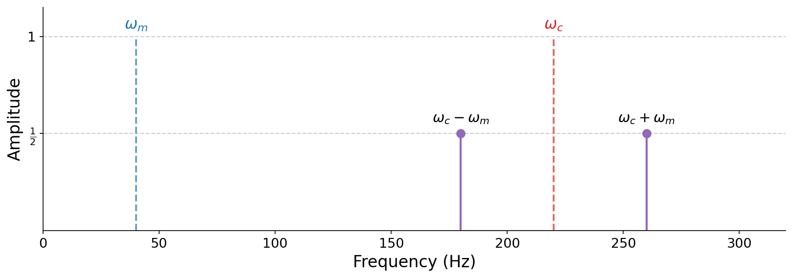
A frequency-domain stem plot. The two input frequencies (modulator at 40 Hz and carrier at 220 Hz) are drawn as faint dashed lines that disappear, while two solid output sidebands appear at 180 and 260 Hz, each with amplitude one half.

Fig. 23 The frequency-domain view of ring modulation. The input frequencies \(\blue{\omega_m}\) and \(\red{\omega_c}\) (dashed) disappear, replaced by two sidebands at \(\purple{\omega_c - \omega_m}\) and \(\purple{\omega_c + \omega_m}\) (solid), each with amplitude \(\tfrac{1}{2}\).#

Note

The minus sign on the upper sideband, \(-\tfrac{1}{2}\cos((\purple{\omega_c + \omega_m})t)\), does not change its amplitude. Since \(-\cos(\theta) = \cos(\theta + \pi)\), the sign is just a phase shift of \(\pi\) radians, which we cannot hear. Both sidebands have amplitude \(\tfrac{1}{2}\) in the amplitude spectrum. We will return to this connection between signs and phase in a moment.

This explains the perceptual shift we heard. When \(\blue{\omega_m}\) is small, the two sidebands \(\purple{\omega_c \pm \omega_m}\) sit very close together (for the 3 Hz example, at 237 and 243 Hz), and our ear fuses them into a single tone that seems to beat, or pulse. As \(\blue{\omega_m}\) grows, the sidebands spread apart (for the 48 Hz example, to 192 and 288 Hz), far enough that our ear resolves them as two separate tones. The underlying mathematics are the same in both cases, but our perception differs! Past a certain threshold of modulation frequency, our perception shifts from tremolo (an “effect” applied to a single tone) to polyphony (two separate tones).

The widget below sweeps the same transition continuously. Drag the modulating frequency up from a slow wobble and listen for the moment one pulsing tone becomes two.

# hide
# no-output
from IPython.utils.capture import capture_output
with capture_output():
    %pip install -q plotly anywidget

import asyncio
import os
import numpy as np
import plotly.graph_objects as go
from plotly.subplots import make_subplots
import ipywidgets as widgets
from IPython.display import Audio
import icm_plotly
from icm_plotly import RED, BLUE, GOLD, IRON, TEAL, STEEL

Drag \(f_m\) from a slow wobble up to an audible rate. On the left, the time axis always spans four cycles of the modulator, and the gray outline is the envelope it traces around the carrier. On the right, the two purple sidebands slide apart around the dashed carrier at 240 Hz. The audio card plays the current setting, so you can hear the moment one pulsing tone becomes two steady ones.

# hide
# autorun
FC, FM0 = 240.0, 3.0                # the chapter's carrier, and a slow start

PURPLE = "#6E3B87"                  # the sideband purple of the chapter's figures

# the time axis always spans four modulator cycles: the window is fixed in
# units of its own length, and only the seconds it stands for change
U = np.linspace(0.0, 1.0, 8000)
MOD = np.sin(2 * np.pi * 4 * U)
ENV = np.abs(MOD)

def window(fm, U=U):
    return U * 4.0 / fm             # seconds

SR = 44100
T_PLAY = np.arange(int(2.5 * SR)) / SR
CARRIER_P = np.sin(2 * np.pi * FC * T_PLAY)

def figure():
    fig = make_subplots(rows=1, cols=2, horizontal_spacing=0.13)
    t = window(FM0)
    fig.add_scatter(x=t * 1000, y=np.sin(2 * np.pi * FC * t) * MOD,
                    mode="lines", line=dict(color=RED, width=1.0),
                    row=1, col=1)
    for sign in (1.0, -1.0):      # the outline sits on top of the band
        fig.add_scatter(x=t * 1000, y=sign * ENV, mode="lines",
                        line=dict(color=IRON, width=1.8, dash="dash"),
                        row=1, col=1)
    fig.add_scatter(x=[FC, FC, None], y=[0, 1.0, None], mode="lines",
                    line=dict(color=RED, width=1.4, dash="dot"), row=1, col=2)
    fig.add_scatter(x=[FM0, FM0, None], y=[0, 1.0, None], mode="lines",
                    line=dict(color=BLUE, width=1.4, dash="dot"),
                    row=1, col=2)
    fig.add_scatter(x=[FC - FM0, FC - FM0, None, FC + FM0, FC + FM0, None],
                    y=[0, 0.5, None, 0, 0.5, None], mode="lines",
                    line=dict(color=PURPLE, width=3.4), row=1, col=2)
    fig.update_xaxes(range=[0, 4000 / FM0], title_text="Time (ms)",
                     fixedrange=True, row=1, col=1)
    fig.update_yaxes(range=[-1.15, 1.15], title_text="Amplitude",
                     fixedrange=True, row=1, col=1)
    fig.update_xaxes(range=[0, 420], title_text="Frequency (Hz)",
                     fixedrange=True, row=1, col=2)
    fig.update_yaxes(range=[0, 1.08], title_text="Magnitude",
                     fixedrange=True, row=1, col=2)
    return fig

def controls(fig):
    fm = widgets.FloatSlider(description="Modulator $f_m$ (Hz)", min=2.0,
                             max=120.0, value=FM0, step=0.5)
    readout = widgets.HTML()

    # the defaults snapshot the arrays; the page's notebooks share one kernel
    def update(fm, window=window, MOD=MOD, FC=FC, readout=readout):
        t = window(fm)
        ms = t * 1000
        with fig.batch_update():
            fig.data[0].x, fig.data[0].y = ms, np.sin(2 * np.pi * FC * t) * MOD
            fig.data[1].x = ms
            fig.data[2].x = ms
            fig.data[4].x = [fm, fm, None]
            fig.data[5].x = [FC - fm, FC - fm, None, FC + fm, FC + fm, None]
            fig.update_xaxes(range=[0, 4000 / fm], row=1, col=1)
        readout.value = (f"<span style='font-size:0.9em'>sidebands at "
                         f"<i>f</i><sub>c</sub> &plusmn; <i>f</i><sub>m</sub> = "
                         f"{FC - fm:.1f} and {FC + fm:.1f} Hz "
                         f"&nbsp;·&nbsp; {2 * fm:.1f} swells per second"
                         f"</span>")

    widgets.interactive_output(update, {"fm": fm})

    # the audio card under the controls: the previous clip stays in place
    # while you drag (so the layout never jumps) and is swapped for the new
    # one when the pointer releases (keyboard nudges settle on a timer). It is
    # written through the Output's synced `outputs` trait, which works
    # outside a kernel message, where display() output has no destination
    out = widgets.Output()
    gate = icm_plotly.release_gate()   # pointer state: is a slider mid-drag?
    pending = []
    dirty = []

    def render(T_PLAY=T_PLAY, CARRIER_P=CARRIER_P, SR=SR):
        x = 0.125 * CARRIER_P * np.sin(2 * np.pi * fm.value * T_PLAY)
        x[:441] *= np.linspace(0, 1, 441)
        x[-441:] *= np.linspace(1, 0, 441)
        audio = Audio(x.astype(np.float32), rate=SR, normalize=False)
        data, metadata = get_ipython().display_formatter.format(audio)
        # one assignment swaps the old card for the new one in place, so
        # the page never shows an empty card and nothing shifts
        out.outputs = ({"output_type": "display_data",
                        "data": data, "metadata": metadata},)


    async def settle():
        await asyncio.sleep(0.25)
        pending.clear()
        if dirty and not gate.dragging:
            dirty.clear()
            render()

    def on_change(_):
        dirty.append(True)
        if pending:
            pending.pop().cancel()
        pending.append(asyncio.ensure_future(settle()))

    def on_release(change):
        if not change["new"] and dirty:
            if pending:
                pending.pop().cancel()
            dirty.clear()
            render()

    gate.observe(on_release, names="dragging")

    for s in (fm,):
        s.observe(on_change, names="value")
    if not os.environ.get("ICM_BOOK_BUILD"):   # the build bakes no card
        render()
    return widgets.VBox([fm, readout, out, gate])

icm_plotly.show(figure, controls)
Modulator \(f_m\) (Hz)3.00
sidebands at fc ± fm = 237.0 and 243.0 Hz  ·  6.0 swells per second