3.2 Additive synthesis

The Fourier series

We claimed above that all periodic sound can be expressed as a sum of basic sinusoids. This is a profound result from mathematics known as the Fourier series:

Definition 6 (Fourier series)

If \(x(t)\) is periodic with fundamental period \(t_0\) and fundamental frequency \(f_0 = 1/t_0\), then \(x(t)\) can be represented as

\[x(t) = a_0 + \sum_{k=1}^{K} a_k \sin(2\pi [k \cdot f_0] \, t + \phi_k),\]

where the frequencies are constrained to integer multiples of \(f_0\).

The proof is beyond the scope of this book, but the implications are central to everything that follows. Some periodic signals require infinitely many terms (e.g., a “perfect” square wave), while others are exact with finitely many (e.g., a sine wave itself is a Fourier series with \(K = 1\)). The key constraint is that the frequencies in the sum are not arbitrary — they must be integer multiples of the fundamental frequency \(f_0\). The \(k\)-th sinusoidal component has frequency \(k \cdot f_0\).

Harmonics

Definition 7 (Harmonic)

In the Fourier series expansion, each sinusoidal component is called a harmonic. Harmonic \(k \in \mathbb{Z}_{>0}\) has frequency \(f_k = k \cdot f_0\), amplitude \(a_k\), and initial phase \(\phi_k\).

It follows that the first harmonic (\(k = 1\)) has frequency equal to the fundamental \(f_0\), the second harmonic (\(k = 2\)) has frequency \(2 f_0\), the third has \(3 f_0\), and so on.

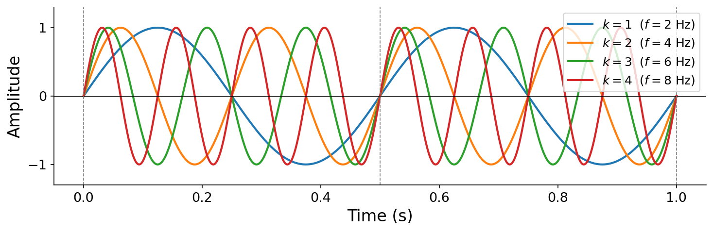
Fig. 4 The first four harmonics of a \(f_0 = 2\) Hz fundamental, all at unit amplitude. Each harmonic \(k\) completes exactly \(k\) cycles per fundamental period. Notice that all harmonics pass through zero together at the fundamental period boundaries (dashed lines) — this is a consequence of the integer frequency constraint.

Note

If you have studied music before, you may have heard “harmonic” and “overtone” used somewhat interchangeably. Despite common conflation, these are not equivalent concepts. Technically, an overtone can take on arbitrary frequencies above the fundamental, not necessarily integer multiples. In this book, we use precise terminology: harmonic \(k\) has frequency \(k \cdot f_0\).

Additive synthesis

In computer music, the Fourier series serves not only as a mathematical expansion but also as a synthesis technique. Additive synthesis builds complex tones by summing sinusoidal harmonics:

Definition 8 (Additive synthesis)

Additive synthesis constructs a periodic tone by summing \(K\) sinusoidal harmonics. Harmonic \(k\) has frequency \(k \cdot f_0\) (an integer multiple of the fundamental frequency \(f_0\)), amplitude \(a_k\), and initial phase \(\phi_k\):

\[x(t) = \sum_{k=1}^{K} a_k \sin(2\pi [k \cdot f_0] \, t + \phi_k)\]

Though the constant \(a_0\) is required for mathematical completeness of the Fourier series, it represents a static offset that is not relevant to our perception of sound, so we ignore it henceforth.

Note

You can think of \(x(t) = a_0\) as a basic sinusoid at \(0\) Hz — the “zeroth harmonic.” We will revisit this when we study the frequency domain.

Synthesis parameters

Synthesis algorithms are often associated with parameters, the constant factors that can be changed to achieve a particular acoustic or creative goal. Additive synthesis has a few parameters:

• \(K\): the highest harmonic number present

• \(f_0\): the fundamental frequency

• \(\mathbf{a} = [a_1, a_2, \ldots, a_K]\): the amplitude coefficients of each harmonic

• \(\boldsymbol{\phi} = [\phi_1, \phi_2, \ldots, \phi_K]\): the initial phase coefficients of each harmonic

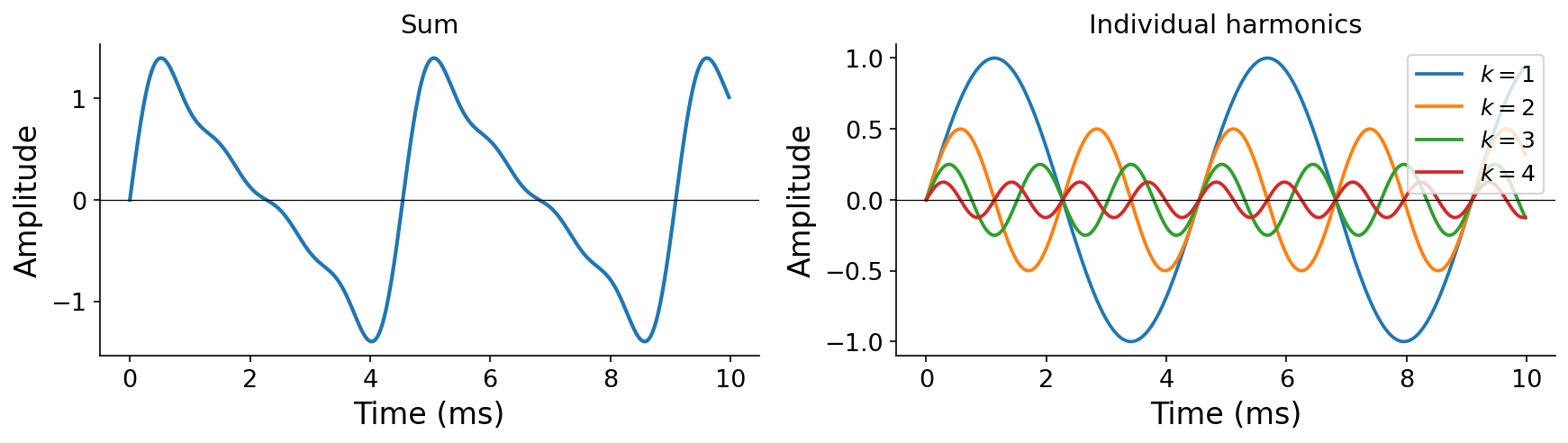
Fig. 5 Additive synthesis with \(K = 4\), \(f_0 = 220\) Hz, \(\mathbf{a} = [1, 1/2, 1/4, 1/8]\). Left: the resulting sum. Right: each harmonic plotted individually — note how each successive harmonic has higher frequency and lower amplitude.

Let’s examine how we perceive each parameter. We’ll use a default tone with \(K = 4\), \(f_0 = 220\) Hz, \(\mathbf{a} = [1, 1/2, 1/4, 1/8]\), and \(\boldsymbol{\phi} = [0, 0, 0, 0]\):

Additive synthesis with \(K = 4\), \(f_0 = 220\) Hz, geometric amplitude decay.

Varying \(f_0\) (pitch): Changing the fundamental frequency shifts all harmonics proportionally and changes the perceived pitch. These four examples all use the same amplitude pattern \(\mathbf{a} = [1, 1/2, 1/4, 1/8]\) but different random fundamental frequencies between 220 and 440 Hz:

Random f0, example 1

Random f0, example 2

Random f0, example 3

Random f0, example 4

Four random fundamental frequencies with the same harmonic amplitude pattern — perceived as different pitches.

Varying amplitudes \(\mathbf{a}\) (timbre): Changing the relative amplitudes of the harmonics changes the timbre — the tonal “color” of a sound. All four examples below have the same pitch (\(f_0 = 220\) Hz) and the same number of harmonics (\(K = 4\)), but different random amplitude patterns produce perceptibly different timbres:

Random timbre 1

Random timbre 2

Random timbre 3

Random timbre 4

Four random amplitude patterns at the same pitch — perceived as different timbres.

Varying phases \(\boldsymbol{\phi}\): Consistent with what we observed for the basic sinusoid, changing the initial phases has very little perceptible effect. The following four examples use the same amplitudes \(\mathbf{a} = [1, 1/2, 1/4, 1/8]\) but different random phases:

Random phase 1

Random phase 2

Random phase 3

Random phase 4

Four random phase patterns with the same amplitudes — sound essentially identical.

These should sound essentially identical, confirming that phase has negligible perceptual effect in additive synthesis. The amplitude coefficients \(\mathbf{a}\) are what matter.

Varying \(K\) (number of harmonics): Adding more harmonics produces a richer, brighter tone. With \(K = 1\) we hear a bare sine wave; as \(K\) grows, the timbre gains complexity:

K = 1

K = 2

K = 4

K = 8

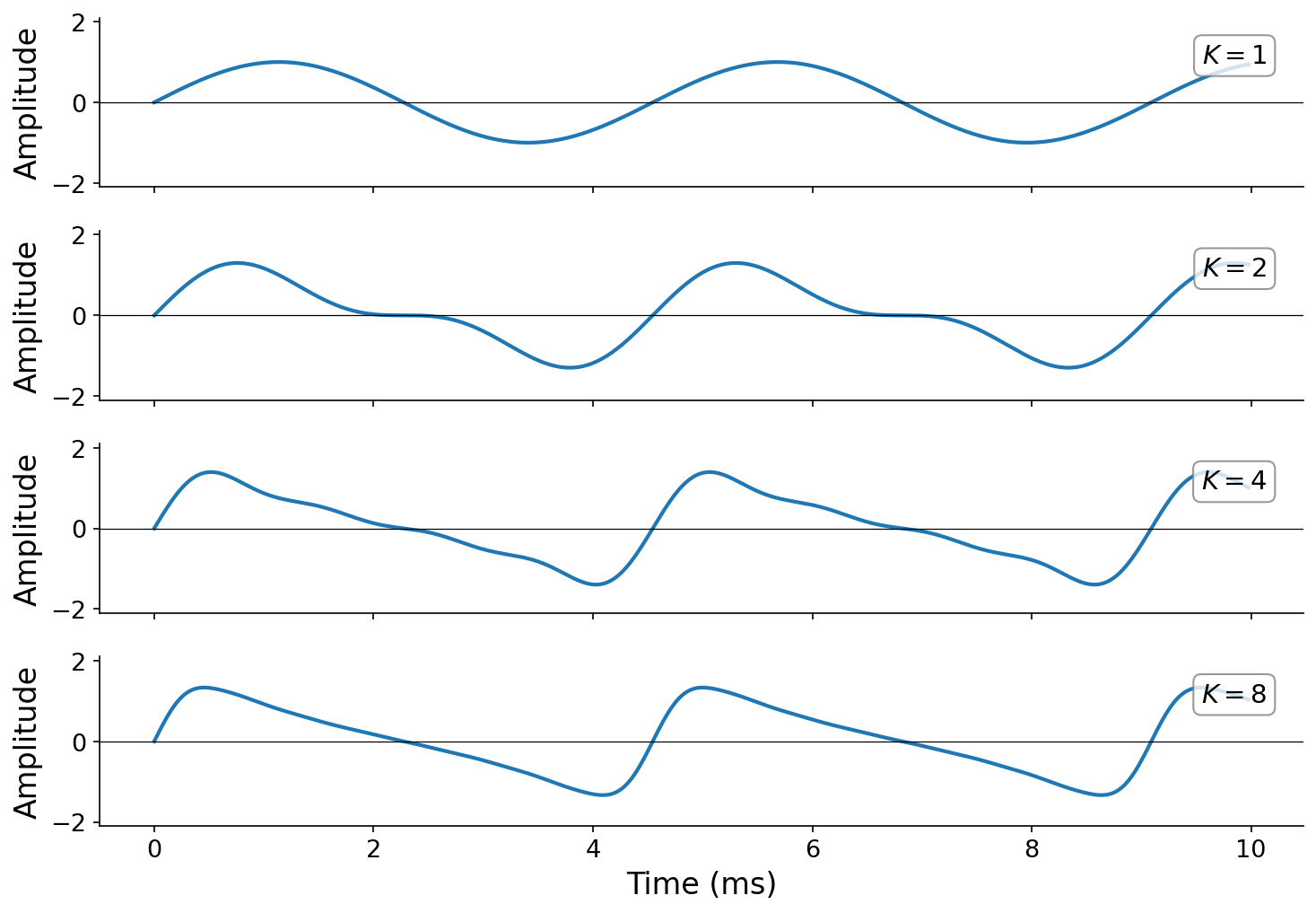
Additive synthesis at \(f_0 = 220\) Hz with \(K \in \{1, 2, 4, 8\}\) harmonics (amplitude pattern \(a_k = 1/2^{k-1}\)). As \(K\) increases, the waveform shape grows more complex and the timbre becomes richer.

The full code for these examples is in code/additive.py.