import matplotlib
if not hasattr(matplotlib.RcParams, "_get"):
    matplotlib.RcParams._get = dict.get

7.4 Quantization and decibels

Sampling is only half the battle in converting continuous sound to digital audio. Recall from Chapter 1 that we must also quantize the real-valued samples so they can be stored in a finite number of bits. Using signed pulse-code modulation with a bit depth of \(b\), we round each amplitude to its nearest representable integer:

\[\hat{x}[n] = \lfloor (2^{b-1} - 1) \cdot x[n] \rfloor.\]

Here is the catch. While audio can be perfectly reconstructed from real-valued samples under the Nyquist condition, quantization is a fundamentally destructive operation. Rounding is many-to-one: distinct amplitudes that round to the same integer become indistinguishable. Quantization introduces an irreversible error, heard as quantization noise.

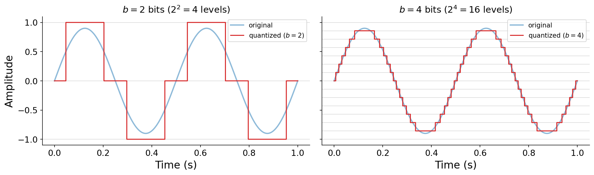
Fig. 41 Quantizing a sine wave at two bit depths. With \(b = 2\) bits (4 levels, left) the staircase is coarse and the error is large. With \(b = 4\) bits (16 levels, right) the error shrinks. Each additional bit doubles the number of levels, halving the error.

How much noise does quantization add, and how many bits do we need to make it inaudible? Before answering, experiment with the effect for yourself. The interactive below (from Chapter 1) quantizes a sine wave at any bit depth: drag \(b\) and watch the staircase coarsen as levels are removed.

# hide
# no-output
from IPython.utils.capture import capture_output
with capture_output():
    %pip install -q plotly anywidget

import asyncio
import os
import numpy as np
import plotly.graph_objects as go
from plotly.subplots import make_subplots
import ipywidgets as widgets
from IPython.display import Audio
import icm_plotly
from icm_plotly import RED, GOLD, STEEL

Drag \(b\): the red staircase is the sine after quantization to \(2^b\) levels, and the gold trace is the error left behind. The audio card underneath always plays the current bit depth.

# hide
# autorun
F0 = 220.0
t = np.linspace(0.0, 2 / F0, 900, endpoint=False)   # two cycles on screen
y = 0.95 * np.sin(2 * np.pi * F0 * t)
sr = 44100
seg = np.arange(sr) / sr                            # one second, for the ear
tone = 0.95 * np.sin(2 * np.pi * F0 * seg)

def quantize(x, b):
    # the chapter's convention: scale to the 2^b integer levels and floor
    L = 2 ** (b - 1) - 1
    return np.floor(L * x) / L

BITS = range(2, 13)
YQ = {b: quantize(y, b) for b in BITS}
ERR = {b: y - YQ[b] for b in BITS}
LEVELS = {}
for b in BITS:
    L = 2 ** (b - 1) - 1
    if b <= 4:                        # level guides only while they are legible
        xs, ys = [], []
        for k in range(-L, L + 1):
            xs += [0, 2000 / F0, None]
            ys += [k / L, k / L, None]
        LEVELS[b] = (xs, ys)
    else:
        LEVELS[b] = ([], [])

def figure():
    fig = make_subplots(rows=2, cols=1, shared_xaxes=True,
                        row_heights=[0.68, 0.32], vertical_spacing=0.1)
    fig.add_scatter(x=LEVELS[3][0], y=LEVELS[3][1], mode="lines",
                    line=dict(color=STEEL, width=1, dash="dot"), row=1, col=1)
    fig.add_scatter(x=t * 1000, y=y, mode="lines",
                    line=dict(color=STEEL, width=1.6), row=1, col=1)
    fig.add_scatter(x=t * 1000, y=YQ[3], mode="lines",
                    line=dict(color=RED, width=2), row=1, col=1)
    fig.add_scatter(x=t * 1000, y=ERR[3], mode="lines",
                    line=dict(color=GOLD, width=1.6), row=2, col=1)
    fig.update_yaxes(range=[-1.15, 1.15], title_text="Amplitude",
                     fixedrange=True, row=1, col=1)
    fig.update_yaxes(range=[0, 1.05], title_text="Error",
                     fixedrange=True, row=2, col=1)
    fig.update_xaxes(fixedrange=True, row=1, col=1)
    fig.update_xaxes(range=[0, 2000 / F0], title_text="Time (ms)",
                     fixedrange=True, row=2, col=1)
    return fig

def controls(fig):
    b = widgets.IntSlider(description="Bit depth b", min=2, max=12, value=3)
    readout = widgets.HTML()

    # the defaults snapshot the arrays; the page's notebooks share one kernel
    def update(b, YQ=YQ, ERR=ERR, LEVELS=LEVELS, readout=readout):
        with fig.batch_update():
            fig.data[0].x, fig.data[0].y = LEVELS[b]
            fig.data[2].y = YQ[b]
            fig.data[3].y = ERR[b]
        L = 2 ** (b - 1) - 1
        readout.value = (f"<span style='font-size:0.9em'>2<sup>{b}</sup> = "
                         f"{2 ** b} levels &nbsp;·&nbsp; spacing 1/{L} "
                         f"≈ {1 / L:.4f}</span>")

    widgets.interactive_output(update, {"b": b})

    # the audio card under the controls: the previous clip stays in place
    # while you drag (so the layout never jumps) and is swapped for the new
    # one when the pointer releases (keyboard nudges settle on a timer). It is
    # written through the Output's synced `outputs` trait, which works
    # outside a kernel message, where display() output has no destination
    out = widgets.Output()
    gate = icm_plotly.release_gate()   # pointer state: is a slider mid-drag?
    pending = []
    dirty = []

    def render(tone=tone, sr=sr, quantize=quantize):
        x = quantize(tone, b.value)
        x *= 0.125 / np.abs(x).max()          # about -18 dBFS, a safe level
        x[:441] *= np.linspace(0, 1, 441)
        x[-441:] *= np.linspace(1, 0, 441)
        audio = Audio(x.astype(np.float32), rate=sr, normalize=False)
        data, metadata = get_ipython().display_formatter.format(audio)
        # one assignment swaps the old card for the new one in place, so
        # the page never shows an empty card and nothing shifts
        out.outputs = ({"output_type": "display_data",
                        "data": data, "metadata": metadata},)

    async def settle():
        await asyncio.sleep(0.25)
        pending.clear()
        if dirty and not gate.dragging:
            dirty.clear()
            render()

    def on_change(_):
        dirty.append(True)
        if pending:
            pending.pop().cancel()
        pending.append(asyncio.ensure_future(settle()))

    def on_release(change):
        if not change["new"] and dirty:
            if pending:
                pending.pop().cancel()
            dirty.clear()
            render()

    gate.observe(on_release, names="dragging")

    b.observe(on_change, names="value")
    if not os.environ.get("ICM_BOOK_BUILD"):   # the build bakes no card
        render()
    return widgets.VBox([b, readout, out, gate])

icm_plotly.show(figure, controls)

Bit depth b3

2³ = 8 levels  ·  spacing 1/3 ≈ 0.3333

Answering our question quantitatively requires a way to reason about amplitude the way our ears do, which brings us to a short but essential detour.

A detour: amplitude perception and the decibel

Human hearing spans an astonishing range of sound pressures. The quietest audible sound corresponds to a pressure fluctuation of about 20 μPa (the threshold of hearing), while the onset of pain occurs around 20 Pa (the threshold of pain). That is a factor of one million: six orders of magnitude between the softest and loudest sounds we can handle. This enormous range is precisely why our perception of loudness is roughly logarithmic rather than linear. A logarithmic response lets us hear both rustling leaves and a roaring engine without any adjustment.

To reason about such a wide range, we need a logarithmic unit. That unit is the decibel (dB). A decibel is one tenth of a bel, and it is fundamentally defined over power \(P\) (the rate at which sound energy is transmitted) relative to a reference power \(P_0\):

\[\text{dB} = 10 \log_{10}\!\left(\frac{P}{P_0}\right).\]

In computer music we usually work with amplitude \(a\), which is proportional to pressure, rather than power. Since power is proportional to the square of amplitude (\(P \propto a^2\)), the square becomes a factor of 2 outside the logarithm:

\[\text{dB} = 10 \log_{10}\!\left(\frac{a^2}{a_0^2}\right) = 20 \log_{10}\!\left(\frac{a}{a_0}\right).\]

Definition 22 (Decibel (amplitude))

The level of an amplitude \(a\) relative to a reference amplitude \(a_0\), expressed in decibels (dB), is

\[\text{dB} = 20 \log_{10}\!\left(\frac{a}{a_0}\right).\]

The decibel is a relative unit: it always compares an amplitude \(a\) to some reference \(a_0\). Two conventions for that reference are common:

• dBFS (decibels relative to full scale) uses \(a_0 = 1\), the maximum amplitude before clipping. So \(\text{dBFS} = 20\log_{10}(a)\). Because amplitudes are at most 1, dBFS values are normally negative, and a value of 0 dBFS means the signal is right at the clipping point.

• dB SPL (sound pressure level) uses the physical reference \(p_0 = 20\) μPa, the threshold of hearing, so \(\text{dB SPL} = 20\log_{10}(p/p_0)\). This grounds the decibel in real-world pressure. It matters less for us in this book, but it connects our unitless amplitudes back to physical sound.

Because the decibel is logarithmic, multiplying an amplitude corresponds to adding decibels. Two relationships are worth committing to memory:

• Multiplying or dividing an amplitude by 10 is a change of \(\pm 20\) dB (since \(20\log_{10}(10) = 20\)).

• Multiplying or dividing an amplitude by 2 is a change of about \(\pm 6\) dB (since \(20\log_{10}(2) \approx 6\)).

With these, we can quickly estimate the dynamic range of human hearing: six orders of magnitude is \(6 \times 20 = 120\) dB. In practice, ambient background noise usually limits the usable range to something closer to 100 dB.

To calibrate your ear to the scale, here is the same 440 Hz sine tone at a ladder of levels, each 20 dB (a factor of 10 in amplitude) below the last:

-6 dBFS

-26 dBFS

-46 dBFS

-66 dBFS

-86 dBFS

A 440 Hz sine at five levels, each 20 dB quieter than the previous (a tenfold drop in amplitude). Even the faintest, at \(-86\) dBFS, is audible on most systems, hinting at the wide dynamic range our ears command. Be careful not to turn your volume up to hear the quiet ones, or the loud ones may surprise you.

Pyquist provides helpers to convert between amplitudes and dBFS:

import pyquist as pq

pq.helper.db_to_amplitude(-6.0)   # ~0.501  (halving amplitude)
pq.helper.db_to_amplitude(-20.0)  # ~0.1    (one tenth amplitude)
pq.helper.amplitude_to_db(0.125)  # ~-18.06 dB

How many bits are enough?

We can now quantify quantization noise in perceptual terms. With \(b\) bits spanning the full-scale range \([-1, 1]\), the spacing between adjacent quantization levels is roughly \(1/2^{b-1}\). If we assume each sample falls at a random point between two levels, the typical rounding error is about half that spacing, or roughly \(1/2^b\).

The key consequence follows immediately. Each time we add one bit, we double the number of levels, which halves the quantization error. And halving an amplitude, as we just learned, is a reduction of about 6 dB. Therefore:

Important

Each additional bit of depth reduces quantization noise by about 6 dB, and so buys about 6 dB of dynamic range.

This gives us a simple rule for choosing a bit depth. At \(b = 16\) bits, we get about \(16 \times 6 = 96\) dB of dynamic range. That is close to the roughly 100 dB practical limit of human hearing, which is exactly why 16 bits per sample (“CD quality”) is enough for transparent audio. It is also conveniently a multiple of 8 bits, aligning with computer word sizes. Professional workflows sometimes use 24 bits to leave extra headroom during editing, but 16 bits is perceptually sufficient for final playback.