import matplotlib
if not hasattr(matplotlib.RcParams, "_get"):
    matplotlib.RcParams._get = dict.get
6.4 Modulating frequency over time#
The modulation techniques so far all center on modulating amplitude over time. They have interesting side effects in the frequency domain, but what if we want to modulate frequency in a more direct way? For example, how would we synthesize vibrato, where a performer wavers the fundamental frequency of their sound over time?
The guitar vibrato from the introduction. On the last note, the performer slides their finger back and forth along the fretboard, causing the pitch itself to fluctuate periodically.
Let us revisit the basic sinusoid, taking unit amplitude and zero initial phase for simplicity:
with angular frequency \(\omega = 2\pi f\) in \(\frac{\text{radians}}{\text{second}}\).
Tip
As always, if you feel rusty with angular frequency, revisit Frequency and angular frequency. We work in angular frequency \(\omega\) here to keep the expressions compact.
To get vibrato, we want the frequency \(\omega\) to change over time, so we replace the constant \(\omega\) with a function \(\omega(t)\). The tempting first attempt is to substitute it directly into the formula:
where \(\Delta t = 1/f_s\) is the sample period. This is wrong. To hear why, let us drive it with a frequency that ramps from 440 Hz up to 880 Hz:
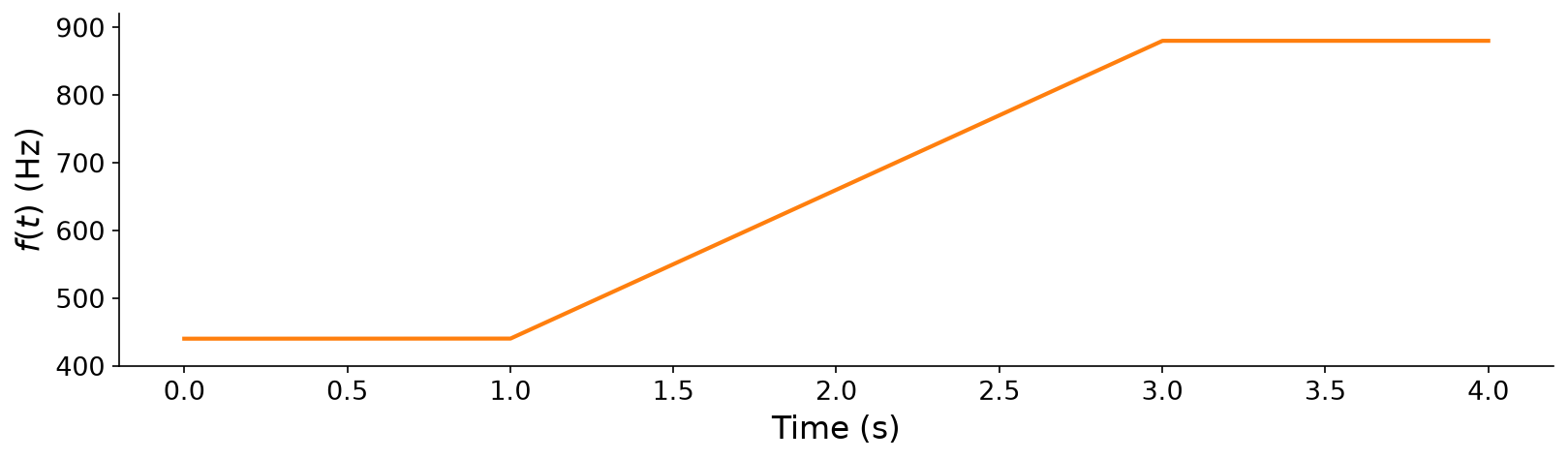
Fig. 27 A time-varying frequency control signal \(f(t)\): 440 Hz held, ramped up to 880 Hz, then held. We will use it to drive both the wrong and the correct time-varying oscillators.#
The same frequency ramp, synthesized two ways. The wrong way has two discontinuous jumps in frequency at the start and end of the ramp up, while the right way ramps smoothly from 440 Hz to 880 Hz.
Why does the naive version fail so badly? The problem is that \(\sin(\omega(t)\cdot t)\) confuses frequency with phase. The argument to \(\sin\) should be the accumulated instantaneous phase, the total number of radians the oscillator has swept out so far. When \(\omega\) is constant, that accumulation is exactly \(\omega t\). But when \(\omega\) changes over time, multiplying the current frequency by the total elapsed time erases history. It retroactively pretends the oscillator was always running at its current frequency.
The fix is to recognize that frequency is a rate of change of phase, so to recover phase we must accumulate (integrate) frequency over time. In continuous terms, we rewrite the basic sinusoid with an integral:
Note
Do not be alarmed by the integral sign. As we noted in Chapter 5, working out closed-form integrals is not a focus of this book. Read the integral at a high level: it simply sums up how much phase has elapsed up to time \(t\). When \(\omega(\tau) = \omega\) is constant, the area under a flat line from \(0\) to \(t\) is just \(\omega t\), recovering the familiar \(\sin(\omega t)\). That equivalence is exactly why we “got away with” the simple form for constant-frequency tones.
On a computer, we cannot evaluate the continuous integral directly. Instead, we approximate it with a Riemann sum. The integral \(\int_0^t \omega(\tau)\,d\tau\) is the area under the frequency curve up to time \(t\), and a Riemann sum estimates that area by slicing it into thin rectangles and adding them up. Each rectangle spans one sample, so it has width \(\Delta t\) and height \(\omega[n]\), contributing a sliver of phase \(\omega[n]\,\Delta t\).
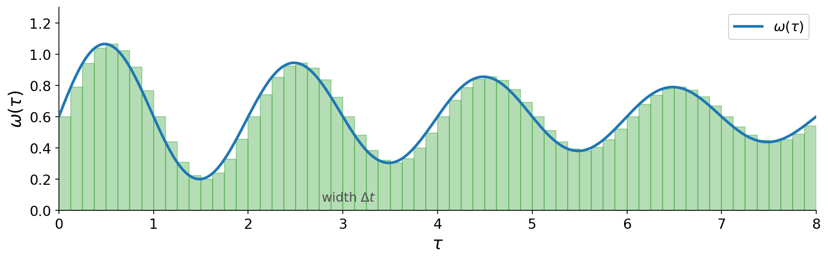
Fig. 28 A Riemann sum approximates the area under a curve by summing the areas of thin rectangles, each of width \(\Delta t\) and height equal to the curve. The narrower the rectangles, the better the approximation. We use this to turn the continuous phase integral into a sum over samples.#
Summing these slivers converts the integral into a discrete sum, exactly as we converted the continuous formula into a sampled one above:
This is now correct, but naively it is also slow. Recomputing the whole sum from scratch for every sample \(n\) would cost \(O(N^2)\) operations. We can do much better by noticing that each phase sum is just the previous one plus a single new term. Naming the accumulated phase \(\theta[n] = \sum_{k=0}^{n}\omega[k]\,\Delta t\), we get a simple recurrence:
This accumulate-a-running-total trick brings the cost back down to \(O(N)\). In fact, the recurrence is exactly a cumulative sum, which NumPy computes for us in a single vectorized call, np.cumsum: given an array \(x\), it returns \(\texttt{cumsum}[n] = \texttt{cumsum}[n-1] + x[n]\) (with \(\texttt{cumsum}[n] = 0\) for \(n < 0\)). So the correct oscillator is simply np.sin(np.cumsum(2 * np.pi * freq / f_s)).
The interactive example below builds the frequency ramp above with np.interp, then synthesizes it both the wrong way (multiplying the current frequency by the total elapsed time) and the correct way (accumulating phase with np.cumsum), so you can hear the difference. Edit the freq control signal and listen:
def osc_naive(freq: np.ndarray, f_s: int = 44100) -> pq.Audio:
    """WRONG: multiply the *current* frequency by the *total* elapsed time."""
    n = np.arange(len(freq))
    theta = 2 * np.pi * freq * n / f_s
    return pq.Audio(np.sin(theta), f_s)


def osc(freq: np.ndarray, f_s: int = 44100) -> pq.Audio:
    """CORRECT: accumulate frequency into phase with np.cumsum, then take sin."""
    theta = np.cumsum(2 * np.pi * freq / f_s)
    return pq.Audio(np.sin(theta), f_s)


f_s = 44100
T = 4.0
t = np.arange(int(T * f_s)) / f_s

# A frequency control signal: 440 Hz held, ramped up to 880 Hz, then held.
# Try editing the breakpoints (times and frequencies) and re-running!
freq = np.interp(t, [0.0, 1.0, 3.0, 4.0], [440.0, 440.0, 880.0, 880.0])

pq.play(osc_naive(freq, f_s))  # the wrong way: discontinuous jumps in pitch
pq.play(osc(freq, f_s))        # the correct way: a smooth sweep
The same comparison as a standalone script is in code/modulation.py. With a correct time-varying oscillator in hand, vibrato is just a matter of choosing \(\omega(\tau)\) to waver gently around a center frequency. That choice is the gateway to frequency modulation.