9.0 What is a filter?#
In signal processing, the word filter is remarkably broad. It refers to essentially any function that takes a signal as input and produces another signal as output. Because signals are themselves functions of time, a filter can be viewed as a function of functions.
In this book we study digital filters. A digital filter is a function \(g\) that maps input samples \(\blue{x}\) to output samples \(\purple{y}\), which we write \(g : \blue{x} \mapsto \purple{y}\):
We can view both the input and output as arrays in \(\mathbb{R}^N\). Accordingly, a digital filter is a mapping between arrays, \(g : \mathbb{R}^N \to \mathbb{R}^N\). This is a deliberately broad definition, and says nothing yet about how a filter is implemented.
This definition is so broad that it covers many familiar topics in computer music:
Some of the synthesis techniques we have already seen, such as modulation synthesis, that transform one signal into another.
Many audio effects you may have encountered outside this book: reverb, delay, distortion, equalization, compression, and so on.
Here we will narrow our attention to an especially important subclass: linear time-invariant (LTI) filters. LTI filters are so ubiquitous in computer music and digital signal processing that the word “filter” is shorthand for LTI filters in colloquial usage. We will define linear and time-invariant precisely later in the chapter. For now, the important thing is their high-level purpose.
The high-level goal of an LTI filter is to sculpt the frequency-domain content of a sound. An LTI filter cannot invent new frequencies. It can only boost or attenuate the frequencies already present in its input, each by an amount that depends on the frequency.
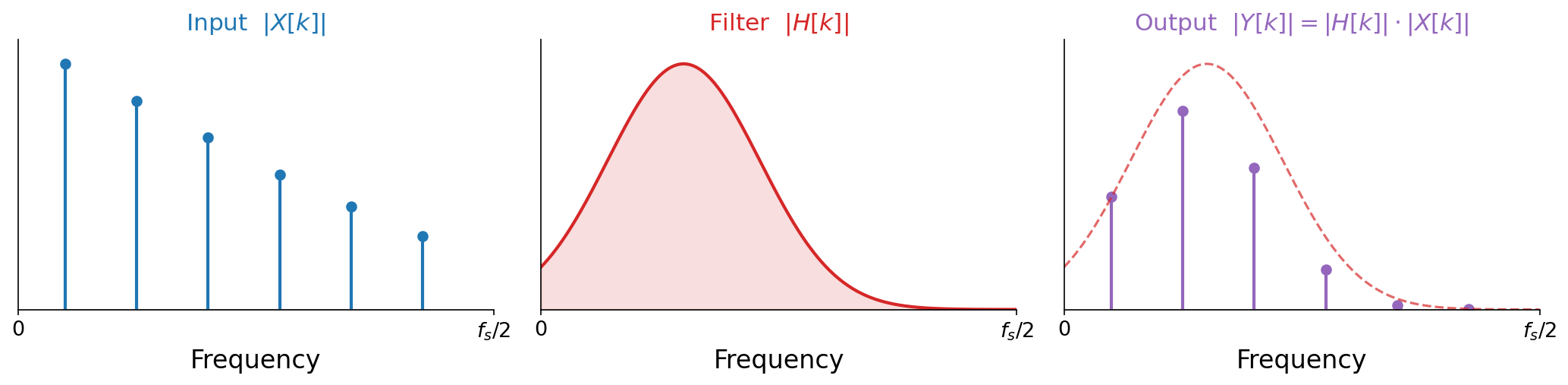
Fig. 48 An LTI filter reshapes a sound in the frequency domain. Each partial of the input \(|X[k]|\) (blue) is scaled by the filter’s response \(|H[k]|\) (red), yielding the output \(|Y[k]| = |H[k]| \cdot |X[k]|\) (purple). The dashed red outline repeats the filter response over the output, showing the ceiling it imposes on the frequency content. No new partials appear, and the existing ones are only reweighted.#
Over the next several sections we will build up several complementary perspectives on LTI filters: difference equations, convolution, impulse responses, frequency-domain multiplication, and signal-flow diagrams. Each perspective focuses on different properties of filters from low-level implementation to high-level behaviors.