2.3 NumPy primer#
Here we provide a basic overview of NumPy. For a more detailed tutorial, we point readers to the official learning resources and the official quickstart tutorial.
Creating arrays#
A NumPy array (a numpy.ndarray) can be built from a Python list:
import numpy as np

x = np.array([0.0, 0.5, 1.0, 0.5, 0.0, -0.5, -1.0, -0.5])
print(x.shape, x.dtype)   # (8,) float64
NumPy arrays have attributes shape and dtype, which respectively define the shape of the array (a simple 1D array in the above example) and the type of data stored within (64-bit floating point numbers).
For audio buffers, we usually allocate by length instead, and optionally fill the initial buffer with some audio material.
zeros = np.zeros(N)                    # a length-N silent buffer
noise = np.random.randn(N) * 0.01      # low amplitude white noise
np.zeros(N) is exactly silence: \(x[n] = 0\) for all \(n\). np.random.randn(N) * 0.01 draws each sample independently from a standard normal distribution and scales it down by a factor of 100; the result is white noise at a low amplitude.
Warning
Headphone warning. Never do computer music programming using headphones. You could seriously damage your ears. Our perception of volume in relation to amplitude is a tricky relationship: just because a signal is in \([-1, 1]\) does not mean it cannot damage your ears. Random and synthesized signals are the most dangerous signals you can play through headphones while learning. A one-character typo (0.01 → 1.0) can turn a quiet hiss into a deafening full-scale roar. Use external speakers at low volume during development.
Slicing arrays#
If you are already familiar with Python list slicing, NumPy supports all the slicing patterns you would expect (they each return np.ndarray):
x = np.arange(10)            # [0, 1, 2, ..., 9]
x[0]                         # 0
x[-1]                        # 9, the last element
x[2:5]                       # [2, 3, 4]
x[::2]                       # [0, 2, 4, 6, 8] - every other element
x[::-1]                      # [9, 8, 7, ..., 0] - reversed
For audio, slicing is how you grab a chunk of a recording. If samples is one second of audio at \(f_s = 44{,}100\), then samples[:22050] is the first half-second and samples[22050:] is the second.
Element-wise operations#
Arithmetic on arrays is element-wise: every operation is applied independently to corresponding elements, with no Python-level loop in sight.
x = np.array([1, 2, 3])
y = np.array([10, 20, 30])

x + y                # [11, 22, 33]
x * y                # [10, 40, 90]
x ** 2               # [1, 4, 9]
np.sqrt(x)           # [1.0, 1.414, 1.732]
Some operations will automatically cast data types for you, e.g., x.dtype above is int64, while np.sqrt(x).dtype is float64.
A NumPy operation between an array and a scalar automatically broadcasts the scalar across every element, i.e., it’s equivalent to creating an array filled with the scalar value:
x + 1                # [2, 3, 4]
0.5 * x              # [0.5, 1.0, 1.5]
This is exactly what happened when we wrote 2 * np.pi * f * (n / f_s) in the previous section: all sample indices in array n (int64) are divided by sample rate f_s to convert them to times (float64), and scalar 2 * np.pi * f is multiplied into the entire n / f_s array in a single expression.
Assignments and in-place operations#
NumPy arrays can be modified after creation. You can assign to individual elements or to whole slices:
samples = np.zeros(N)              # silent buffer of length N
samples[100] = 0.5                 # set a single sample
samples[:1000] = 1.0               # set the first 1000 samples to 1.0
samples[1000:2000] = np.sin(...)   # fill a slice with another array
NumPy also supports the compound arithmetic operators (+=, -=, *=, /=). On arrays these update the existing array in place, rather than allocating a new one. Compare the two ways to halve every sample of a buffer:
# Out-of-place: allocates a new array; the original `samples` is unchanged
result = samples * 0.5

# In-place: updates `samples` directly, no new allocation
samples *= 0.5
The in-place form is usually faster and more memory-efficient, since there’s no fresh array to allocate, fill, and (eventually) garbage-collect. Slice targets work too, which is handy for mixing additional material into part of an existing buffer:
samples[:1000] += other # mix `other` into the first 1000 samples in place
Multi-channel arrays and stereo audio#
Arrays in NumPy can be multidimensional. The arrays we’ve looked at so far are 1D vectors, but NumPy arrays can represent 2D matrices or even higher-dimensional structures. Two helpful attributes characterize an array’s layout:
arr.ndim: the number of dimensions (1 for a vector, 2 for a matrix, …).arr.shape: a tuple giving the size along each dimension.
v = np.array([1.0, 2.0, 3.0])
v.ndim, v.shape                  # 1, (3,)

m = np.array([[1.0, 2.0], [3.0, 4.0], [5.0, 6.0]])
m.ndim, m.shape                  # 2, (3, 2)
Music is often rendered in stereo: two arrays of samples (often called channels), one for each ear, which allows for basic spatial effects. We represent a stereo signal as a 2D NumPy array.
There are two reasonable orderings: time-major (num_samples, num_channels) and channel-major (num_channels, num_samples). We will adopt the time-major convention (num_samples, num_channels) throughout this book and in the Pyquist library (introduced in the next section).
A small example: one second of stereo audio with a 220 Hz tone in the left channel and a 330 Hz tone in the right.
f_s = 44100
N = f_s
n = np.arange(N)
t = n / f_s

left  = 0.5 * np.sin(2 * np.pi * 220 * t)   # shape (N,)
right = 0.5 * np.sin(2 * np.pi * 330 * t)   # shape (N,)

stereo = np.stack([left, right], axis=1)    # shape (N, 2)
print(stereo.shape)                         # (44100, 2)
np.stack(..., axis=1) glues two length-\(N\) arrays side by side along a new axis at position 1, producing the time-major (N, 2) layout.
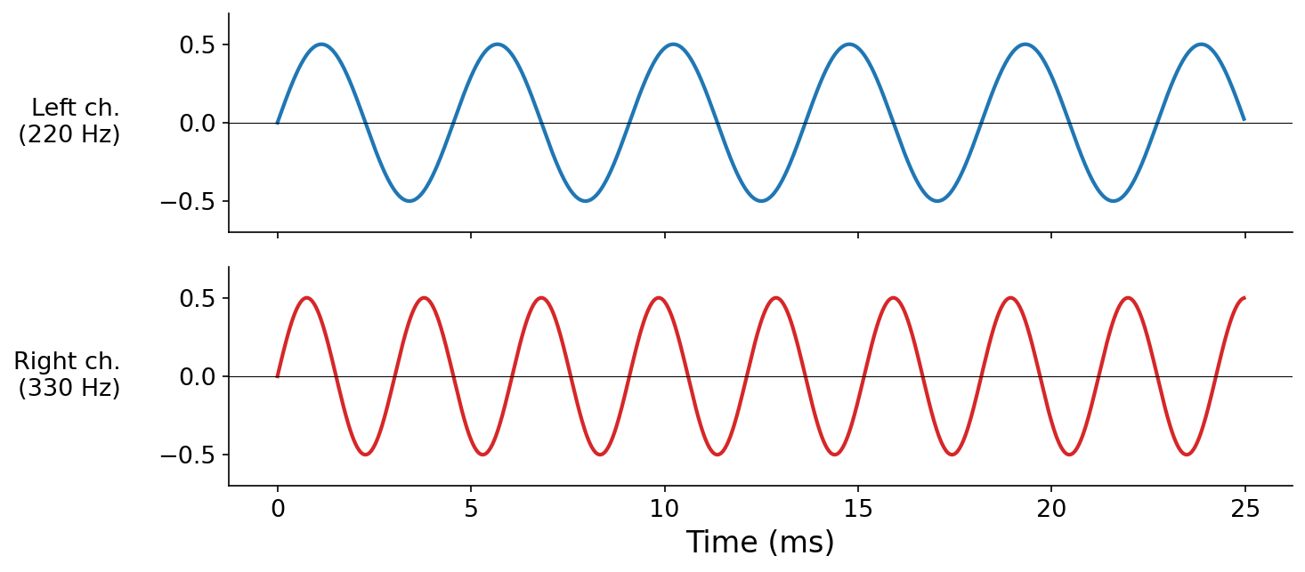
One second of stereo audio: 220 Hz in the left channel, 330 Hz in the right channel. (Best heard with stereo speakers or, cautiously, with headphones.)
Slicing a 2D array uses commas to address each axis:
stereo[:, 0]             # the left channel only (1D, shape (N,))
stereo[:, 1]             # the right channel only
stereo[:1000, :]         # the first 1000 samples of both channels (2D, shape (1000, 2))
stereo[:1000]            # equivalent shorthand
Broadcasting#
The np.stack trick above works, but a more elegant pattern scales up to more channels. NumPy’s broadcasting rules let us combine arrays of different shapes, provided the shapes are compatible.
An example in music synthesis: let’s say we wanted to synthesize stereo audio consisting of two sine waves with a different frequency in the left and right channel. To do this, we implicitly want to evaluate sine at all points in time and at two different frequencies, i.e., a nested loop. Using NumPy’s broadcasting rules, we can concisely represent these types of multi-dimensional operations:
# In vanilla Python as a nested loop
freqs = [220.0, 330.0]
stereo = [[0.0, 0.0] for _ in range(N)]      # N distinct [left, right] rows
for n in range(N):
    t = n / f_s
    for c in range(2):
        stereo[n][c] = 0.5 * math.sin(2 * np.pi * freqs[c] * t)

# As vectorized / broadcasted operations in NumPy
t = np.arange(N) / f_s
freqs = np.array(freqs)
# t[:, np.newaxis] has shape (N, 1)
# freqs            has shape (2,)
# Their product broadcasts to shape (N, 2)
stereo = 0.5 * np.sin(2 * np.pi * freqs * t[:, np.newaxis])
np.newaxis adds an axis of length 1, reshaping t from (N,) to (N, 1). NumPy then aligns the two shapes from the right ((N, 1) vs. (2,)), and where one shape has a 1, it stretches (broadcasts) that array along that axis. The result has shape (N, 2), identical to the np.stack version above.
To go from stereo back to mono, average across the channel axis:
mono = stereo.mean(axis=1) # shape (N,)
The same stereo example, downmixed to mono by averaging the two channels. Both pitches are present in a single channel.
Tip
If you didn’t completely follow this broadcasting example, don’t worry. Mastering multidimensional operations and broadcasting rules in NumPy requires practice, and you will naturally gain experience throughout this course.