1.2 From analog to digital

1.2 From analog to digital#

Computers cannot store an analog signal \(x(t)\) directly. The function takes real-valued inputs and produces real-valued outputs, so even a one-second clip carries an infinite amount of information. To bring sound into the digital world, we have to approximate \(x(t)\) with a finite amount of data. The pipeline that performs this approximation is called analog-to-digital conversion (ADC).

Transforming this continuous sound to digital audio involves discretizing both time and amplitude:

Sampling in time: measure the signal amplitude at discrete, evenly spaced points known as samples.
Quantizing in amplitude: latch each amplitude to its nearest neighbor in a finite set of amplitude values.

Sampling#

Definition 1 (Sampling)

To sample a continuous signal means to measure or evaluate it at a sequence of discrete time points, uniformly spaced at some interval \(\Delta t\).

We call \(\Delta t\) the sampling period; its units are \(\frac{\text{seconds}}{\text{sample}}\). Its reciprocal \(f_s\), in units of \(\frac{\text{samples}}{\text{second}}\), is called the sample rate. The sample rate represents the number of samples captured per second, and the units reveal that \(f_s = 1 / \Delta t\). Sample rates of 44,100 Hz and 48,000 Hz are common values of \(f_s\) in practice; that is, digital audio usually involves tens of thousands of samples per second.

We index samples by an integer \(n\) and adopt the convention

\[x[n] = x(n \Delta t) = x(n / f_s),\]

so \(x[0]\) is the signal at time \(t = 0\), \(x[1]\) is its value at time \(t = 1 \cdot \Delta t\), and so on. Continuous-time signals get parentheses (\(x(t)\)); discrete-time sample sequences get square brackets (\(x[n]\)). This distinction will matter throughout the book. You should grow very accustomed to converting between \(\text{samples}\) and \(\text{seconds}\) by dividing or multiplying by \(f_s\).

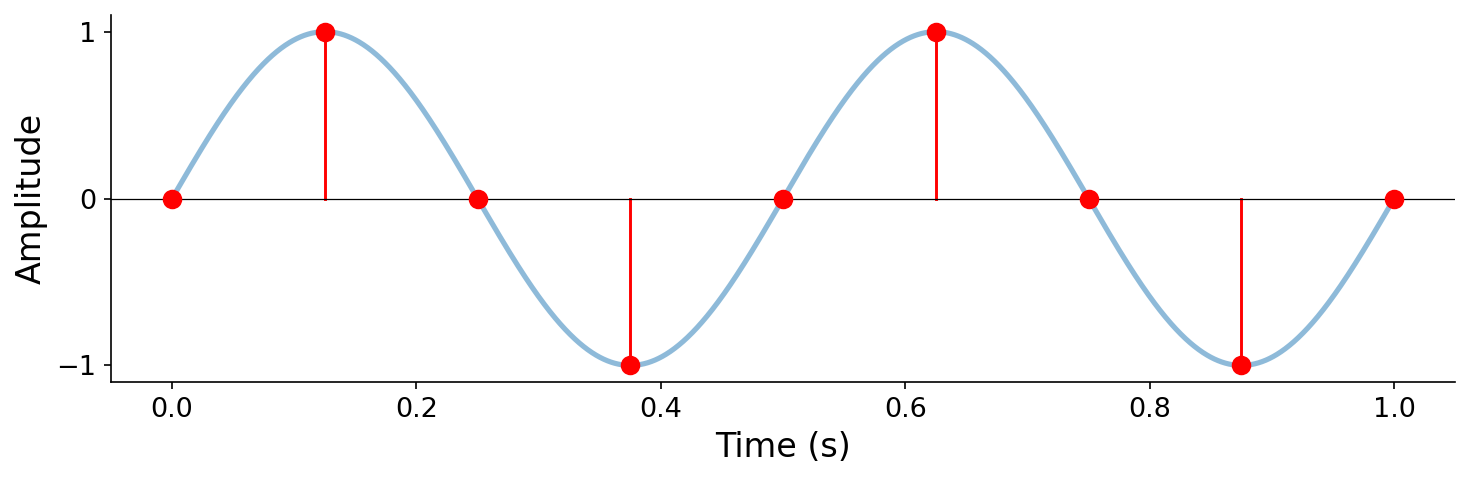
A continuous sine wave with discrete sample points marked as red dots connected to the horizontal axis by vertical lines, illustrating sampling at 8 samples per second

After sampling, an infinite continuous function has been replaced by a finite ordered sequence of real numbers. Specifically, for some duration \(T\), \(x\) is now a array of numbers of length \(T \cdot f_s\), i.e., \(x \in \mathbb{R}^{T \cdot f_s}\). But the values \(x[n]\) are still real-valued, and we still cannot store real numbers exactly.

Quantization#

Sampling shrank time from a continuum to a finite grid, but we have an analogous problem in amplitude. The values \(x[n] \in \mathbb{R}\) are still real-valued, and a computer cannot store an arbitrary real number exactly.

Definition 2 (Quantization)

To quantize a sample is to latch its amplitude to a nearby element of a finite set of amplitude values.

A common quantization convention in digital audio is signed pulse-code modulation (PCM). We pick an integer bit depth \(b\) and define

\[\mathbb{Z}_b = \{-2^{b-1},\, -2^{b-1}+1,\, \ldots,\, 2^{b-1}-1\}\]

as the set of \(2^b\) integers representable in \(b\) bits using two’s complement. We then map each amplitude \(x[n] \in [-1, 1]\) to its quantized integer counterpart by scaling and truncating:

\[\hat{x}[n] = \lfloor (2^{b-1} - 1) \cdot x[n] \rfloor \in \mathbb{Z}_b.\]

For example, at \(b = 16\) (“CD quality”), \(\mathbb{Z}_{16}\) contains the \(2^{16} = 65{,}536\) integers between \(-32{,}768\) and \(32{,}767\), and amplitudes of \(\{-1.0, 0.0, 1.0\}\) correspond to integers \(\{-32767, 0, 32767\}\) respectively (\(-32768\) is unused).

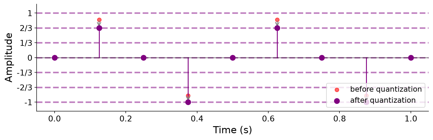
Sample points before and after quantization to three-bit signed PCM (the eight levels of the set Z_3), with dashed horizontal lines showing the representable amplitude levels and arrows indicating the flooring of each sample down to the representable level at or below it

Quantization is lossy: any two amplitudes that floor to the same integer become indistinguishable in \(\hat{x}[n]\). We will study and quantify the impacts of amplitude quantization when we cover quantization and decibels in more detail.

The interactive below quantizes a sine wave at any bit depth. Drag \(b\) and watch the staircase coarsen.

# hide
# no-output
from IPython.utils.capture import capture_output
with capture_output():
    %pip install -q plotly anywidget

import asyncio
import os
import numpy as np
import plotly.graph_objects as go
from plotly.subplots import make_subplots
import ipywidgets as widgets
from IPython.display import Audio
import icm_plotly
from icm_plotly import RED, GOLD, STEEL

Drag \(b\): the red staircase is the sine after quantization to \(2^b\) levels, and the gold trace is the error left behind. The audio card underneath always plays the current bit depth.

# hide
# autorun
F0 = 220.0
t = np.linspace(0.0, 2 / F0, 900, endpoint=False)   # two cycles on screen
y = 0.95 * np.sin(2 * np.pi * F0 * t)
sr = 44100
seg = np.arange(sr) / sr                            # one second, for the ear
tone = 0.95 * np.sin(2 * np.pi * F0 * seg)

def quantize(x, b):
    # the chapter's convention: scale to the 2^b integer levels and floor
    L = 2 ** (b - 1) - 1
    return np.floor(L * x) / L

BITS = range(2, 13)
YQ = {b: quantize(y, b) for b in BITS}
ERR = {b: y - YQ[b] for b in BITS}
LEVELS = {}
for b in BITS:
    L = 2 ** (b - 1) - 1
    if b <= 4:                        # level guides only while they are legible
        xs, ys = [], []
        for k in range(-L, L + 1):
            xs += [0, 2000 / F0, None]
            ys += [k / L, k / L, None]
        LEVELS[b] = (xs, ys)
    else:
        LEVELS[b] = ([], [])

def figure():
    fig = make_subplots(rows=2, cols=1, shared_xaxes=True,
                        row_heights=[0.68, 0.32], vertical_spacing=0.1)
    fig.add_scatter(x=LEVELS[3][0], y=LEVELS[3][1], mode="lines",
                    line=dict(color=STEEL, width=1, dash="dot"), row=1, col=1)
    fig.add_scatter(x=t * 1000, y=y, mode="lines",
                    line=dict(color=STEEL, width=1.6), row=1, col=1)
    fig.add_scatter(x=t * 1000, y=YQ[3], mode="lines",
                    line=dict(color=RED, width=2), row=1, col=1)
    fig.add_scatter(x=t * 1000, y=ERR[3], mode="lines",
                    line=dict(color=GOLD, width=1.6), row=2, col=1)
    fig.update_yaxes(range=[-1.15, 1.15], title_text="Amplitude",
                     fixedrange=True, row=1, col=1)
    fig.update_yaxes(range=[0, 1.05], title_text="Error",
                     fixedrange=True, row=2, col=1)
    fig.update_xaxes(fixedrange=True, row=1, col=1)
    fig.update_xaxes(range=[0, 2000 / F0], title_text="Time (ms)",
                     fixedrange=True, row=2, col=1)
    return fig

def controls(fig):
    b = widgets.IntSlider(description="Bit depth b", min=2, max=12, value=3)
    readout = widgets.HTML()

    # the defaults snapshot the arrays; the page's notebooks share one kernel
    def update(b, YQ=YQ, ERR=ERR, LEVELS=LEVELS, readout=readout):
        with fig.batch_update():
            fig.data[0].x, fig.data[0].y = LEVELS[b]
            fig.data[2].y = YQ[b]
            fig.data[3].y = ERR[b]
        L = 2 ** (b - 1) - 1
        readout.value = (f"<span style='font-size:0.9em'>2<sup>{b}</sup> = "
                         f"{2 ** b} levels &nbsp;·&nbsp; spacing 1/{L} "
                         f"≈ {1 / L:.4f}</span>")

    widgets.interactive_output(update, {"b": b})

    # the audio card under the controls: the previous clip stays in place
    # while you drag (so the layout never jumps) and is swapped for the new
    # one when the pointer releases (keyboard nudges settle on a timer). It is
    # written through the Output's synced `outputs` trait, which works
    # outside a kernel message, where display() output has no destination
    out = widgets.Output()
    gate = icm_plotly.release_gate()   # pointer state: is a slider mid-drag?
    pending = []
    dirty = []

    def render(tone=tone, sr=sr, quantize=quantize):
        x = quantize(tone, b.value)
        x *= 0.125 / np.abs(x).max()          # about -18 dBFS, a safe level
        x[:441] *= np.linspace(0, 1, 441)
        x[-441:] *= np.linspace(1, 0, 441)
        audio = Audio(x.astype(np.float32), rate=sr, normalize=False)
        data, metadata = get_ipython().display_formatter.format(audio)
        # one assignment swaps the old card for the new one in place, so
        # the page never shows an empty card and nothing shifts
        out.outputs = ({"output_type": "display_data",
                        "data": data, "metadata": metadata},)

    async def settle():
        await asyncio.sleep(0.25)
        pending.clear()
        if dirty and not gate.dragging:
            dirty.clear()
            render()

    def on_change(_):
        dirty.append(True)
        if pending:
            pending.pop().cancel()
        pending.append(asyncio.ensure_future(settle()))

    def on_release(change):
        if not change["new"] and dirty:
            if pending:
                pending.pop().cancel()
            dirty.clear()
            render()

    gate.observe(on_release, names="dragging")

    b.observe(on_change, names="value")
    if not os.environ.get("ICM_BOOK_BUILD"):   # the build bakes no card
        render()
    return widgets.VBox([b, readout, out, gate])

icm_plotly.show(figure, controls)

Bit depth b3

2³ = 8 levels · spacing 1/3 ≈ 0.3333

A signal sampled at \(f_s\) samples per second and quantized to \(b\) bits per sample has a bitrate

\[\text{bitrate} \left[\frac{\text{bits}}{\text{seconds}}\right] = f_s \left[ \frac{\cancel{\text{samples}}}{\text{second}} \right] \cdot b \left[ \frac{\text{bits}}{\cancel{\text{sample}}} \right].\]

For so-called “CD-quality” audio (\(f_s = 44{,}100\), \(b = 16\)), that is \(44{,}100 \cdot 16 = 705{,}600 \left[\frac{\text{bits}}{\text{seconds}}\right]\). To get a more intuitive sense of file size, we can convert to kilobytes per second by chaining the standard relationships \(8\,\text{bits} = 1\,\text{byte}\) and \(1000\,\text{bytes} = 1\,\text{kilobyte}\):

\[705{,}600 \left[\frac{\cancel{\text{bits}}}{\text{seconds}}\right] \cdot \frac{1}{8} \left[\frac{\cancel{\text{byte}}}{\cancel{\text{bits}}}\right] \cdot \frac{1}{1000} \left[\frac{\text{kilobyte}}{\cancel{\text{byte}}}\right] \approx 88 \left[\frac{\text{kilobytes}}{\text{seconds}}\right].\]

A three-minute song therefore occupies roughly \(88 \cdot 180 \approx 16\) megabytes on disk in this uncompressed form.

Most music is stored and reproduced in stereo, meaning there are two arrays or channels (one for each of our ears) that allow us to perceive basic music spatialization. This doubles the storage size, resulting in \(1{,}411{,}200 \left[\frac{\text{bits}}{\text{seconds}}\right]\) for stereo CD-quality audio. Note that, unless otherwise specified, we are usually referring to mono (single channel) digital audio in this text.

Digital audio is just an array of numbers!#

The punchline here is that, when stored on disk in formats like WAV, digital audio is basically just an array of numbers (samples) together with the sample rate.

When stored on disk, these numbers are usually integers. Why integers and not floats? A 32-bit floating-point number reserves a large fraction of its 32 bits for representing very large and very small magnitudes, i.e., values far outside \([-1, 1]\) that audio simply never uses. The audible range \([-1, 1]\) is a thin sliver of float’s representable range, so most of those bits go to waste on every sample. Integer PCM, by contrast, packs every bit into uniform amplitude resolution inside \([-1, 1]\), giving more precision per bit of storage.

When synthesizing or manipulating samples in memory, the conventions differ. When you write computer music programs, you’ll almost always manipulate \(x[n]\) as a floating-point number in \([-1, 1]\) for arithmetic convenience: mixing, filtering, and synthesis all involve multiplication, addition, and transcendental functions that are awkward and lossy in integer space. Quantization typically only enters the picture at the boundary, when reading samples from a sound file or writing them out.