import matplotlib
if not hasattr(matplotlib.RcParams, "_get"):
    matplotlib.RcParams._get = dict.get

10.4 The short-time Fourier transform

Granular synthesis showed that frame-based processing can do genuinely creative things. Now we turn to perhaps its most powerful application: the short-time Fourier transform (STFT), which reveals how a sound’s frequency content evolves over time.

Recall the limitation of the DFT: it integrates over all time, turning \(N\) samples into \(N\) bins and, in the process, discarding when each frequency occurred. But of course frequency content changes over time in music, that is what a musical melody is. How can we see those changes? The idea is exactly the frame-based recipe: slice the signal into frames and take the DFT of each one.

Definition 31 (Short-time Fourier transform)

The short-time Fourier transform of a signal \(x\) applies the DFT to each extracted frame:

\[\texttt{STFT}_k(x) = \texttt{DFT}(x_k), \qquad x_k[n] = x[k \cdot N_H + n].\]

For a signal of \(N\) samples with hop length \(N_H\) and frame length \(N_F\), the output is a complex matrix of shape \(\frac{N}{N_H} \times N_F\): one row per frame, one column per frequency bin (or \(\frac{N_F}{2}+1\) columns for real-valued audio).

Taking the magnitude of each frame and stacking the frames side by side gives a spectrogram, a two-dimensional image with time on the horizontal axis, frequency on the vertical axis, and amplitude encoded as color intensity. Because our ears perceive amplitude roughly logarithmically, we usually take the \(\log\) of the magnitude before mapping it to color. For the same reason, the frequency axis is often drawn on a log scale too: our sense of pitch is logarithmic, so an octave (a doubling of frequency) sounds like a constant step no matter where it falls, and a log axis gives every octave equal space. We will develop this logarithmic view of pitch in Chapter 15.

The spectrogram is one of the most important visualizations in all of audio. Here it is on a simple rising melody, C-D-E-F-G played as sine tones, shown three ways for comparison:

The C-D-E-F-G melody

The same rising C-D-E-F-G melody shown three ways: in symbolic form (top), as a log-frequency spectrogram (middle), and as a plain DFT of the whole signal (bottom). The DFT finds all five pitches but loses their order; the spectrogram shows each pitch at the moment it sounds, so the rising melody is unmistakable.

The plain DFT sees all five notes as five peaks but cannot tell you their order. The spectrogram shows each note stepping up in turn. That extra time axis is the whole point of the STFT.

The STFT is really just the frame-based recipe with a DFT in the middle: cut the signal into frames, and take the DFT of each one.

Fig. 69 The STFT as analysis: each frame is sent through its own DFT, and the resulting spectra, stacked side by side, form the spectrogram.

Configuring the frame length

The STFT has two key parameters, the frame length \(N_F\) and the hop length \(N_H\), and choosing them well is something of an art. Consider \(N_F\) first. What happens as we make frames longer?

The upside is better frequency resolution. Recall that the DFT bin spacing is \(\Delta f = f_s / N_F\), so longer frames pack the bins closer together and resolve nearby frequencies more finely. But this comes at a cost in time resolution: a longer frame smears a wider stretch of time into a single spectrum. In the extreme where \(N_F\) grows to the whole signal length \(N\), we are back to a single all-of-time DFT, having thrown away time entirely. This is a fundamental trade-off, and you can watch it play out by sweeping \(N_F\) through powers of two:

Fig. 70 The time-frequency resolution trade-off. At the beginning of the animation, short frames give sharp timing but coarse frequency; by the end, long frames give fine frequency detail but blur events together in time.

There is a second cost: computation. Under the FFT, a single DFT of length \(N_F\) costs \(O(N_F \log N_F)\), and the STFT computes one for each of its \(\frac{N}{N_H}\) frames:

\[\underbrace{\frac{N}{N_H}}_{\text{number of frames}} \cdot \underbrace{O(N_F \log N_F)}_{\text{cost per DFT}} \;=\; O\!\left(N \cdot N_F \log N_F\right),\]

taking the hop \(N_H\) to be a constant factor in the last step. So the total cost grows with the frame length \(N_F\), another reason not to make frames larger than the application needs.

There is no universally best \(N_F\); it depends on the application. A few rules of thumb: use a power of two for FFT efficiency, and make the frame at least one cycle of the lowest frequency you care about. The lower limit of human hearing is around \(20\) Hz, a cycle of which is \(\frac{1}{20}\) seconds or \(50\) ms, and at \(44.1\) kHz a \(4096\)-sample frame (\(\approx 93\) ms) comfortably covers it.

Configuring the hop length

The hop length \(N_H\) is a gentler knob. Unlike \(N_F\), it does not affect frequency resolution at all: the DFT of each frame is unchanged no matter how far apart the frames sit. Instead, \(N_H\) controls two things. The first is time resolution, since a smaller hop means more frames per second and a finer-grained view of how the sound changes. The second is computational cost: an STFT of \(N\) samples produces \(\frac{N}{N_H}\) frames, so halving the hop doubles the number of DFTs we must compute.

We usually express the hop as an amount of overlap, the quantity \(\frac{N_F - N_H}{N_F}\) we defined at the start of the chapter. Recall that we must keep \(N_H \le N_F\) or we will skip samples between frames. In the STFT, a common choice is \(N_H = N_F / 2\) (50% overlap), and heavy overlaps like 75% (\(N_H = N_F/4\)) are typical when reconstruction quality matters.

Windowing revisited

We can now settle the question we deferred earlier: why bother with smooth windows? The answer is spectral leakage, which we first met in Chapter 8. Extracting a frame is a multiplicative operation: it is equivalent to multiplying the signal by a rectangular window that is one over the frame and zero everywhere else. By the convolution theorem from Chapter 9, multiplying by a window in time convolves the signal’s spectrum with the window’s spectrum, smearing each sharp spectral line into a blur.

The rectangular window’s spectrum is a sinc function with tall side lobes, so it smears energy far and wide:

Fig. 71 Framing with a rectangular window causes strong spectral leakage. By the convolution theorem, the spectrum of the windowed signal (bottom right) is the signal’s spectrum convolved with the window’s spectrum (a sinc with large side lobes), smearing each sharp line across many bins.

Because every frame is a windowed slice, this leakage is present in every STFT, and it is worse than in a plain DFT because each frame is shorter. The fix is to multiply each frame by a window with a gentler spectrum, such as the Hann window. Its spectrum concentrates energy in a narrow central lobe with much smaller side lobes, so the smearing is greatly reduced:

Fig. 72 A Hann window has a much cleaner spectrum than the rectangle, its side lobes are far smaller, so convolving with it (windowing each frame) reduces spectral leakage substantially.

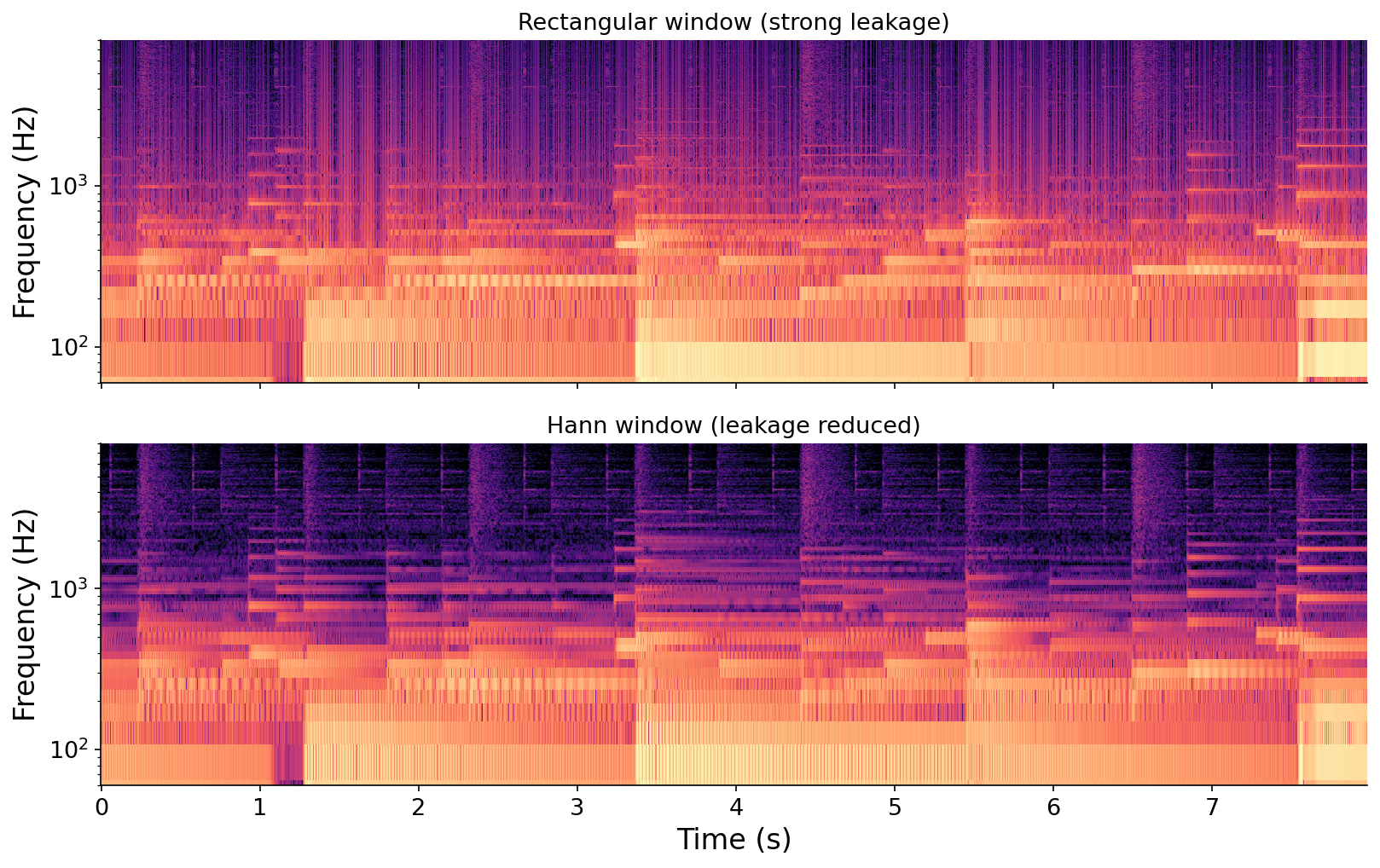
The effect is visible in the spectrogram itself, where the rectangular window’s leakage shows up as vertical smearing that the Hann window cleans away:

Fig. 73 Log-frequency spectrograms of the running example with a rectangular window (top) and a Hann window (bottom). The Hann window’s reduced leakage yields a noticeably cleaner picture.

This is also why granular synthesis windowed each grain: the same smoothing that reduces spectral leakage also removes the audible clicks at grain edges. In the STFT, where we window every frame repeatedly, it is especially important.

Spectral analysis

The spectrogram is a powerful analysis tool. Suppose we are handed the C-D-E-F-G recording from earlier and asked which pitches it contains and when. We can march through the STFT frame by frame, find the loudest frequency in each frame whose energy exceeds some threshold, round it to the nearest musical pitch, and emit a note whenever the detected pitch changes. This turns a pq.Audio into a pq.Score, a crude form of music transcription:

# hide
from typing import Iterator
import numpy as np
import pyquist as pq


def iter_frames(audio: pq.Audio, N_H: int, N_F: int) -> Iterator[np.ndarray]:
    for start in range(0, len(audio) - N_F + 1, N_H):
        yield audio.samples[start:start + N_F]


def overlap_add(frames: np.ndarray, N_H: int, sample_rate: int) -> pq.Audio:
    num_frames, N_F, num_channels = frames.shape
    out = np.zeros((N_H * (num_frames - 1) + N_F, num_channels), dtype=frames.dtype)
    for k, frame in enumerate(frames):
        out[k * N_H:k * N_H + N_F] += frame
    return pq.Audio(out, sample_rate)

from pyquist.helper import frequency_to_pitch

# A tiny monophonic transcriber: for each frame, find the loudest frequency,
# round it to the nearest musical pitch, and emit a note when the pitch changes.
audio = pq.Audio.from_file("./assets/audio-melody.wav")
sr = audio.sample_rate
N_F, N_H = 4096, 1024

# One magnitude spectrum per frame: window each frame, then take its DFT.
frames = np.array(list(iter_frames(audio, N_H, N_F)))[:, :, 0]   # (num_frames, N_F), mono
S = np.abs(np.fft.rfft(frames * np.hanning(N_F), axis=1))
freqs = np.fft.rfftfreq(N_F, 1 / sr)
seconds_per_frame = N_H / sr
threshold = 0.05 * S.max()

events, current, onset = [], None, 0.0
for k in range(len(S)):
    if S[k].max() < threshold:                   # silence
        pitch = None
    else:
        pitch = int(round(frequency_to_pitch(freqs[np.argmax(S[k])])))
    if pitch != current:                         # the note changed
        if current is not None:
            events.append((onset, {"pitch": current, "duration": k * seconds_per_frame - onset}))
        current, onset = pitch, k * seconds_per_frame
if current is not None:                          # flush the final note
    events.append((onset, {"pitch": current, "duration": len(S) * seconds_per_frame - onset}))

score = pq.Score(events)
for event in score:
    print(f"t = {event.time:4.2f}s   MIDI pitch {event.kwargs['pitch']}")

t = 0.00s   MIDI pitch 60
t = 0.46s   MIDI pitch 62
t = 0.98s   MIDI pitch 64
t = 1.46s   MIDI pitch 65
t = 1.97s   MIDI pitch 67

Transcription in general is a hard problem, especially for polyphonic music where many notes sound at once, but this simple peak-picking approach works well enough for clean, monophonic input like our sine melody.

The inverse STFT

We have been computing the STFT; now let us invert it. Is the STFT invertible? We already know the DFT is, since \(x = \texttt{IDFT}(\texttt{DFT}(x))\). So under a rectangular window at 0% overlap, where the frames tile the signal exactly, the STFT is invertible too: applying the inverse DFT to each frame recovers that frame, and overlap-add stitches the frames back together,

\[\texttt{ISTFT}(\texttt{STFT}(x)) = x.\]

Intuitively, the exact invertibility of the DFT implies that the STFT does not change the reconstruction properties of standard frame-based processing. Accordingly, For other windows and overlaps, the same COLA condition from before guarantees perfect reconstruction: as long as the (squared) windows sum to a constant, the inverse DFTs overlap-add back to the original signal (potentially with a constant amplitude gain that we can adjust for). A runnable STFT and inverse STFT are in code/stft.py.

Spectral processing

The invertibility of the STFT unlocks a whole family of effects. We can transform a sound into the time-frequency domain, edit the spectral coefficients however we like, and transform back, a technique called spectral processing. Now that we have analysis and synthesis in hand, the whole pipeline is a single frame-based flow with an editing step in the middle:

Fig. 74 The full STFT pipeline. Analysis (the STFT) frames the signal and takes the DFT of each frame; synthesis (the inverse STFT) takes the inverse DFT of each frame and overlap-adds the results. Editing the spectra in between is spectral processing.

Three quick examples. First, we can apply a brick-wall low-pass filter by simply zeroing out every bin above a cutoff frequency in every frame, which mutes the high end. Second, we can keep each frame’s magnitudes but replace its phases with random values, which smears the sound’s sharp transients into a wash. Third, we can perform cross-synthesis, imposing the spectral envelope of one sound onto another: we keep the trio’s own (complex) spectrum but scale each bin by the magnitude of a voice recording, so the trio takes on the voice’s changing formants, a “talking instrument” effect.

Brick-wall low-pass (bins above 1 kHz zeroed)

Phase randomized (transients smeared)

Cross-synthesis (trio shaped by a speaking voice)

Three spectral-processing effects, all computed by editing the STFT and inverting it. The cross-synthesis multiplies the trio’s spectrum by the magnitude spectrum of a spoken clip (Alvin Lucier’s I Am Sitting in a Room), so the trio is modulated by the voice’s formants.

There is an enormous space of effects to explore here. Try inventing your own by editing the STFT directly:

# hide
import numpy as np
import pyquist as pq


def hann(n):
    return 0.5 * (1 - np.cos(2 * np.pi * np.arange(n) / n))


def stft(x, N_H, N_F, window):
    return np.array([np.fft.rfft(x[s:s + N_F] * window)
                     for s in range(0, len(x) - N_F + 1, N_H)])


def istft(S, N_H, N_F, window):
    out = np.zeros(N_H * (S.shape[0] - 1) + N_F)
    wsum = np.zeros_like(out)
    for k in range(S.shape[0]):
        out[k * N_H:k * N_H + N_F] += np.fft.irfft(S[k], N_F) * window
        wsum[k * N_H:k * N_H + N_F] += window ** 2
    return out / np.maximum(wsum, 1e-8)

# Spectral processing: transform to the time-frequency domain with the STFT,
# EDIT the complex coefficients, and transform back. Try your own edits!
audio = pq.Audio.from_file("./assets/audio-trio.wav")
x = np.asarray(audio.samples).reshape(-1)
sr = audio.sample_rate
N_F, N_H = 2048, 512
w = hann(N_F)

S = stft(x, N_H, N_F, w)          # S is complex, shape (num_frames, num_bins)

# --- edit here --- (this example keeps the magnitudes but randomizes the phases)
magnitude = np.abs(S)
phase = np.random.uniform(-np.pi, np.pi, S.shape)
S = magnitude * np.exp(1j * phase)
# -----------------

y = istft(S, N_H, N_F, w)
pq.play(pq.Audio(y.astype(np.float32), sr))

The phase vocoder

We end our discussion of the STFT with a famous spectral-processing algorithm, the phase vocoder, which performs high-quality time stretching without pitch shifting.

Despite the name, the phase “vocoder” is applied to all kinds of audio, not just voice. It is the algorithm behind the “2x speed” button on video sites. It was originally proposed in 1966 as a low-bandwidth way to transmit speech, one year after the FFT was invented, and the name stuck.

Granular synthesis already gave us pitch-preserving time stretching. But we can also frame time stretching as a spectral-processing operation: to slow a sound to half speed, we want an output STFT with twice as many frames, so we simply interpolate between the input frames. Let’s define \(X[j] = \texttt{STFT}_j(x)\), i.e., the DFT of the \(j\)-th frame of \(x\). For output frame \(i\), we blend input frames \(j = \lfloor i/2 \rfloor\) and \(j+1\):

\[Y[i] = (1 - a)\, X[j] + a\, X[j+1], \qquad a = \tfrac{i}{2} - j.\]

This is not unlike the interpolation operation in wavetable synthesis except applied to complex-valued frames instead of wavetable samples. This sounds reasonable, but it has a subtle flaw involving phase. Each STFT bin has a phase, and when we interpolate we are implicitly assuming we know how that phase advances from one frame to the next. But the phase is only known modulo \(2\pi\): if a bin’s phase reads \(\pi/4\) in one frame and \(5\pi/4\) in the next, did it advance by \(\pi\), or by \(3\pi\), or by \(5\pi\)? The sliding-window nature of the STFT makes this ambiguous, and naive interpolation between ambiguous phases produces a smeared, “phasey” artifact.

Fig. 75 The trouble with phase. A bin’s phase jumps from \(\pi/4\) to \(5\pi/4\) between frames, but the true advance could be \(\pi\), \(3\pi\), \(5\pi\), or any of infinitely many possibilities. The STFT alone cannot disambiguate them.

The phase vocoder resolves this by predicting how the phase should evolve. Bin \(k\) corresponds to a frequency of \(\omega_k\) radians per sample, so over a single hop of \(N_H\) samples its phase should advance by an expected amount of \(\omega_k \cdot N_H\) radians. The algorithm compares this expected advance to the observed advance (the actual phase difference between two consecutive frames) and resolves the \(2\pi\) ambiguity by picking whichever multiple lands nearest the expectation. Accumulating these corrected advances frame by frame builds a clean, continuous phase for the output. The details are beyond our scope, but the result is time stretching that exceeds the quality of granular synthesis:

Original

Half speed (pitch preserved)

Double speed (pitch preserved)

Pitched down an octave (phase vocoder + resampling)

The phase vocoder stretches time while holding pitch constant, and combined with resampling it gives independent control over both.