import matplotlib
if not hasattr(matplotlib.RcParams, "_get"):
    matplotlib.RcParams._get = dict.get
13.4 All-pass filters#
When a sound is played in a room, it bounces off the walls, the floor, and everything in between. Each reflection arrives at a slightly different time, from a slightly different direction, and with a different attenuation. The result is reverberation: thousands of overlapping, delayed copies of the sound. We can see them in the impulse response of a real room, like the church whose impulse response we used for convolution reverb in Chapter 9:
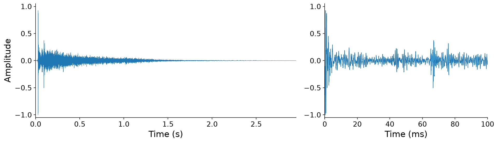
Fig. 101 The impulse response of a church, in full (left) and over its first \(100\) ms (right). After the direct sound, the first reflections arrive as distinct spikes, which soon blur together into thousands of overlapping echoes that decay over about \(2\) seconds. Impulse response from Freesound: IR_Church_01 by snapssound, License: Attribution 4.0.#
Could we simulate reverberation with feedback delay lines? There are two issues. First, a feedback delay line is a comb filter, which colors the sound by imposing the pitch of its teeth, rather than sounding like a room. Second, a realistic reverb needs a huge number of echoes, and so a huge number of delay lines. We could instead use the convolution reverb of Chapter 9, but it requires recording the impulse response of a real room, so it is limited to rooms we have access to.
The solution is a different building block. Recall from Chapter 9 that an all-pass filter leaves the amplitude of every frequency untouched, and alters only its phase. Here is a simple all-pass filter built around a delay line:
Definition 39 (All-pass filter)
The all-pass filter with a delay of \(M \in \mathbb{Z}_{>0}\) samples and a gain \(|g| < 1\) is the recursive filter
Its magnitude response is \(|H(f)| = 1\) at every frequency \(f\), while its phase response \(\angle H(f)\) varies with frequency.
Compared to a feedback delay line, an all-pass filter adds an inverted feedforward term, \(-g \cdot x[n]\), which exactly cancels out the peaks and valleys of the comb:
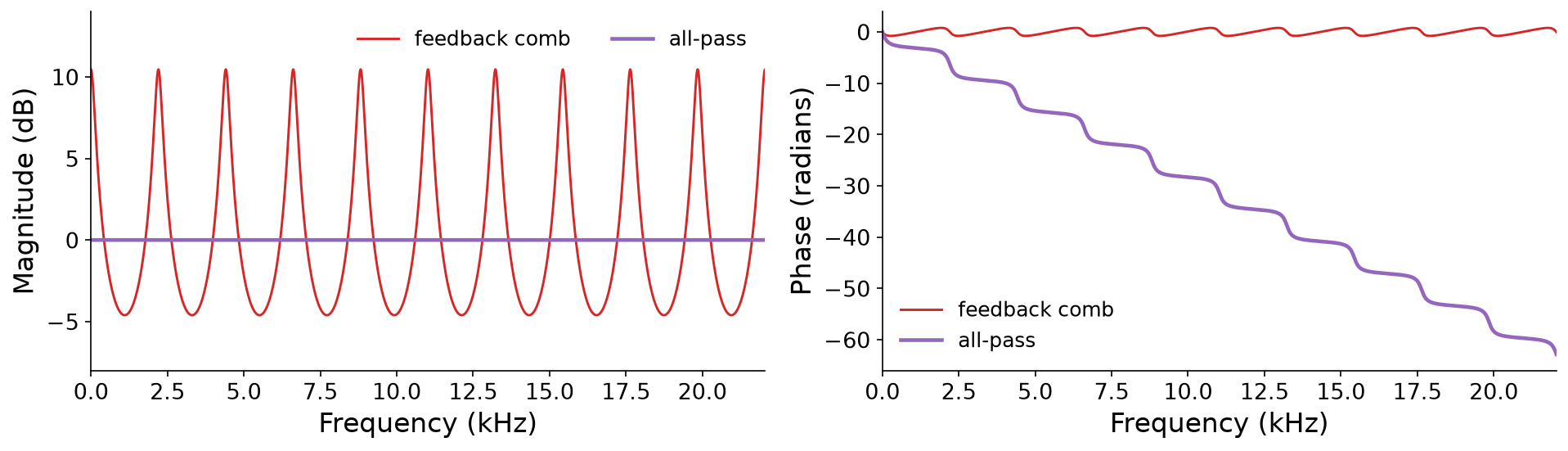
Fig. 102 The magnitude responses (left) and phase responses (right) of a feedback comb filter and an all-pass filter, both with \(M = 20\) and \(g = 0.7\).#
So an all-pass filter does not color the spectrum of a sound. But its impulse response is still a train of echoes, \(h = [-g, 0, \ldots, 0, 1 - g^2, 0, \ldots, 0, g(1 - g^2), \ldots]\), spaced \(M\) samples apart. And when we chain all-pass filters in series, their echoes multiply: each echo of the first filter is echoed again by the second. A short chain of all-pass filters can therefore produce dense echoes without coloring the sound.
We can build an all-pass filter from our feedback delay line. If \(v[n] = x[n] + g \cdot v[n - M]\) is the output of a feedback delay line, then \(y[n] = -g \cdot v[n] + v[n - M]\) is the output of an all-pass filter.
def allpass(x: np.ndarray, M: int, g: float) -> np.ndarray:
    """An all-pass filter, y[n] = -g * x[n] + x[n - M] + g * y[n - M],
    built from a feedback delay line."""
    v = feedback_delay(x, M, g)                          # v[n] = x[n] + g * v[n - M]
    v_delayed = np.concatenate([np.zeros(M), v[:-M]])    # v[n - M]
    return -g * v + v_delayed


impulse = np.zeros(10)
impulse[0] = 1.0
print(np.round(allpass(impulse, M=3, g=0.5), 4))

# Every frequency passes through with a magnitude of 1
long_impulse = np.zeros(44100)
long_impulse[0] = 1.0
h = allpass(long_impulse, M=441, g=0.7)
magnitude = np.abs(np.fft.rfft(h))
print(f"magnitude response: between {magnitude.min():.4f} and {magnitude.max():.4f}")
[-0.5     0.      0.      0.75    0.      0.      0.375   0.      0.
  0.1875]
magnitude response: between 1.0000 and 1.0000
Reverb#
In 1962, Manfred Schroeder combined feedback delay lines and all-pass filters into one of the first artificial reverberators [Sch62]. His design passes the input through four feedback delay lines in parallel, which provide the echoes, and then through two all-pass filters in series, which scatter the echoes into a dense tail:
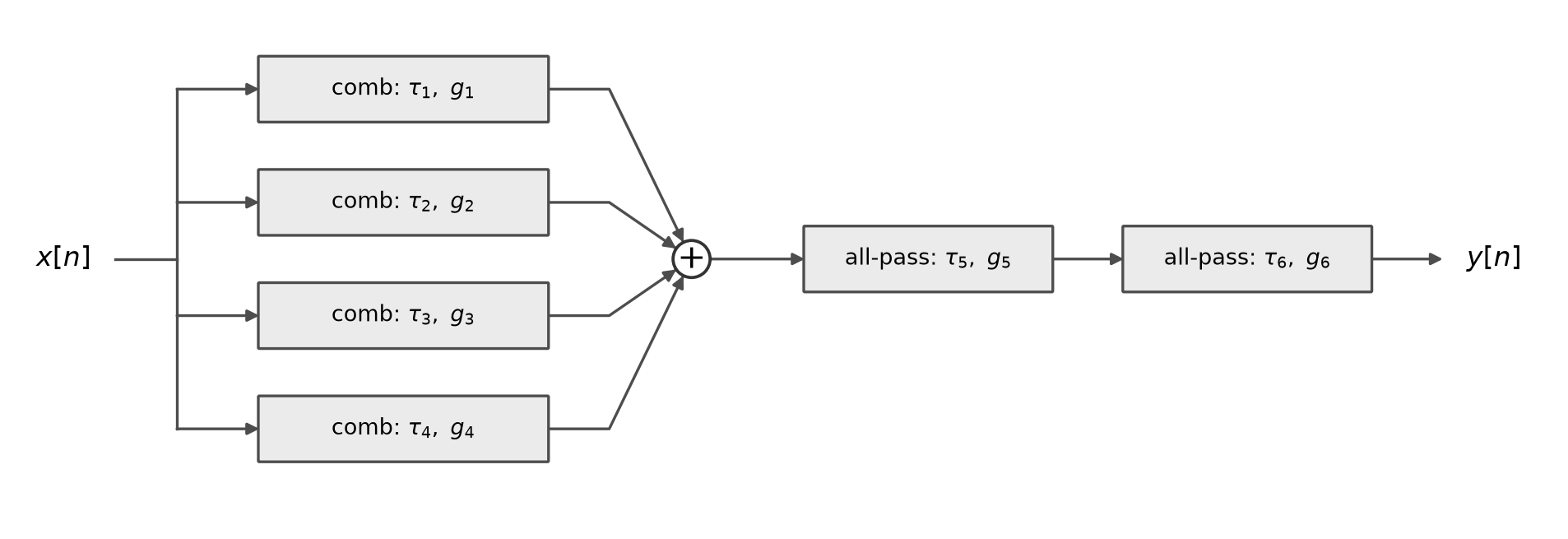
Fig. 103 Schroeder’s reverberator: four feedback comb filters in parallel, followed by two all-pass filters in series. Each block has its own delay \(\tau_k\), in seconds, and gain \(g_k\). After Fig. 6 of [Sch62].#
Schroeder chose comb delays between about \(30\) and \(45\) ms that do not share common factors, so that their echoes do not line up, and short all-pass delays with gains around \(0.7\). A classic set of values is comb delays of \(29.7\), \(37.1\), \(41.1\), and \(43.7\) ms, and all-pass delays of \(5.0\) and \(1.7\) ms. How should we set the gains of the combs? A reverb is usually specified by its reverberation time, \(T_{60}\): the time it takes the reverb to decay by \(60\) dB. This is exactly the setting from Chapter 12, so each comb with a delay of \(M\) samples needs a gain of
The code below implements Schroeder’s reverberator with a reverberation time of \(2\) seconds, using our feedback delay line and all-pass filter, and applies it to the marimba loop from the convolution reverb example of Chapter 9:
def schroeder_reverb(x: np.ndarray, t60: float, f_s: int) -> np.ndarray:
    """Schroeder's reverberator: four feedback combs in parallel, then two
    all-pass filters in series."""
    wet = np.zeros(len(x))
    for tau in [0.0297, 0.0371, 0.0411, 0.0437]:         # comb delays, in seconds
        M = round(tau * f_s)
        g = 10 ** (-3 * M / (f_s * t60))                   # decay by 60 dB in t60 seconds
        wet += (feedback_delay(x, M, g) - x) / 4           # keep only the reflections
    for tau in [0.005, 0.0017]:                           # all-pass delays, in seconds
        wet = allpass(wet, round(tau * f_s), g=0.7)
    return wet


marimba = pq.Audio.from_file("./assets/marimba.wav")
f_s = marimba.sample_rate
x = np.concatenate([marimba.samples[:, 0], np.zeros(2 * f_s)])   # room for the reverb's tail
wet = schroeder_reverb(x, t60=2.0, f_s=f_s)
w = wet_ratio(0.0)
pq.play(marimba, normalize=True)
pq.play(pq.Audio((1 - w) * x + w * wet, f_s), normalize=True)
Most artificial reverbs today still use the same principles, as networks of feedback delay lines and all-pass filters in various topologies.
Sound from Freesound: Marimba loop 3 by BrickDeveloper171, License: CC0.