15.2 Lossy compression#
We now arrive at the key question for this chapter: how can we leverage observations from psychoacoustics to improve codecs, by removing perceptually redundant information?
In this section, we will explore lossy codecs, whose round trip is imperfect:
Our goal is for the distortion to be imperceptible to human ears, as it was for amplitude quantization. Lossy music compression formats (like MP3 and Ogg Vorbis files) can achieve compression factors around \(10\times\) relative to uncompressed CD-quality audio (\(1411\) kbps), with nearly imperceptible distortion. This is remarkable! About \(9\) out of every \(10\) bits that we use to store digital audio are redundant from the perspective of human perception of music. How is this possible?
First, test your ears. Below are three versions of the same drum loop: one uncompressed (\(1411\) kbps), one compressed to MP3 at \(128\) kbps (a compression factor of \(11\times\)), and one compressed to MP3 at \(64\) kbps (\(22\times\)). Which is which?
Reveal the answer
Version 1 is the MP3 at \(128\) kbps, version 2 is uncompressed, and version 3 is the MP3 at \(64\) kbps. Listen for the sizzle of the hi-hats in version 3, whose highest frequencies have been removed.
Unless you’re an unusually sensitive listener, you probably had a difficult time distinguishing between the uncompressed audio and the MP3 with \(11\times\) smaller file size. It turns out that musical sound has two sources of redundancy that codecs can exploit in the frequency domain: perceptual redundancy and statistical redundancy.
Critical bands and masking#
The first source of redundancy is perceptual. The inner ear decomposes sound into roughly \(24\) overlapping frequency bands, called critical bands. Each band is narrow at low frequencies (about \(100\) Hz wide) and wider at high frequencies (several kHz wide), roughly in proportion to our logarithmic perception of pitch. We can emulate them with a filterbank of \(24\) band-pass filters [Zwi61]. Applying the filterbank to every frame of a spectrogram gives a much coarser representation of sound, with just \(24\) “frequencies”:

Fig. 123 A filterbank of \(24\) triangular filters, one per critical band (top), and a drum loop represented as a spectrogram (bottom left) and by the energy in each critical band (bottom right).#
When several frequencies coexist within the range of a critical band, our perception has limited ability to distinguish between them. Specifically, louder frequencies mask quieter ones, making them harder or impossible to hear. There are several kinds of masking.
Frequency masking. A loud tone, the masker, raises the threshold of hearing for other tones in its critical band, and to a lesser extent in neighboring bands. In each example below, a steady \(1000\) Hz masker plays, while a quieter \(1100\) Hz probe beeps three times. First, set your volume so that the masker in the first example is comfortable. That example then plays the quietest probe (\(-40\) dB) on its own, with no masker. Then, in the other examples, how many beeps can you hear?
Masker, then probe alone (−40 dB)

A \(1000\) Hz masker and a \(1100\) Hz probe, at three levels relative to the masker. On its own, the probe is audible even at \(-40\) dB. With the masker, it falls below the masking threshold (dashed, schematic).
Temporal masking. A loud sound can also mask quieter sounds that occur shortly after it ends (and, to a lesser extent, shortly before it begins). In each example below, a \(1000\) Hz masker plays for half a second, followed by a short, quiet probe at the same frequency, \(40\) dB quieter, after different gaps. In the first example, the gap is long enough that the probe should be easy to hear. Can you hear the probe in the others?

A \(1000\) Hz masker, followed by a \(30\) ms probe at \(-40\) dB after three gaps. The masking threshold (dashed, schematic) decays over the \(100\) to \(200\) ms after the masker ends.
The absolute threshold. Finally, recall from the equal-loudness contours that the threshold of hearing depends on frequency. Even with no masker at all, quiet sounds at frequencies where we are less sensitive are inaudible. To hear this, play the \(4000\) Hz tone below, and turn your volume down until it is barely audible. Then, without changing your volume, play the \(8000\) Hz tone, which has the same amplitude (\(-40\) dBFS). (Afterwards, remember to turn your volume back up.)
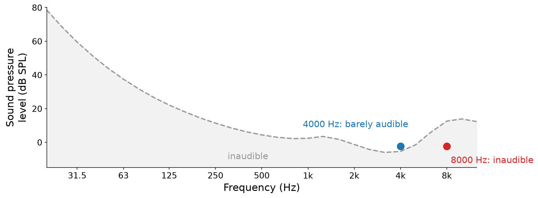
Two tones at the same level, against the threshold of hearing. Once the \(4000\) Hz tone is barely audible, the \(8000\) Hz tone falls about \(15\) dB below the threshold.
Important
When frequencies cannot be perceived, whether because of masking or the absolute threshold, we can remove them from the spectrum. Removing them introduces distortion, but distortion that we cannot hear.
Lossy codecs do exactly this. Below are spectrograms of a guitar recording before and after MP3 compression at \(128\) kbps. Throughout the MP3’s spectrogram, the codec has replaced quiet frequency content (mostly above \(5\) kHz) with zeros, which show up as black holes. It has also removed everything above about \(16\) kHz, where our sensitivity is lowest:
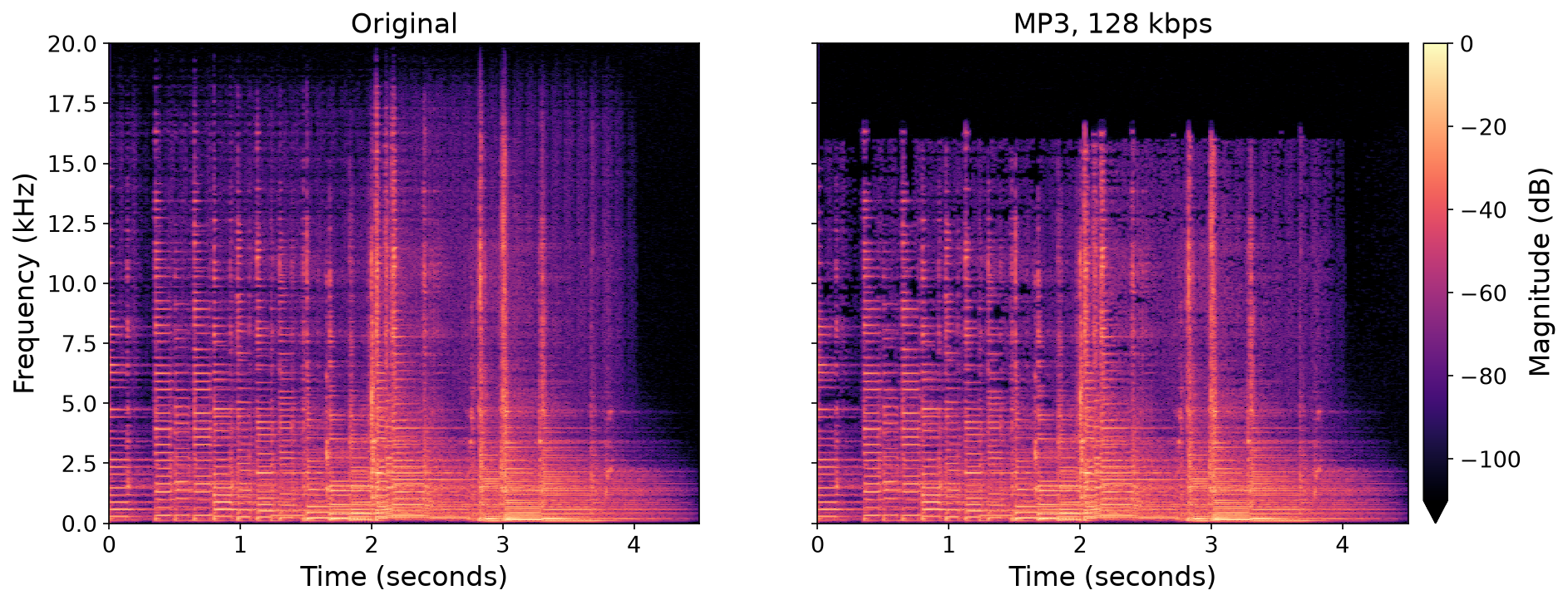
Fig. 124 Spectrograms of a guitar recording, original (left) and as an MP3 at \(128\) kbps (right). Black regions are zero. Recording from Freesound: 388954 by FullMetalJedi, License: CC0.#
Sparsity in frequency#
What should we do with all of these zeros? Compress them! This brings us to the second source of redundancy, which is statistical.
Example: runs of zeros. Say that we need to store strings of \(32\) bits, which we expect to contain very long runs of \(0\)s, for example,
We could store each string verbatim, with \(32\) bits. Or, we could store the lengths of its runs of \(0\)s. This string consists of \(12\) zeros, a one, \(16\) zeros, a one, and a final \(2\) zeros. Every run has at most \(31\) zeros, so we can store each run length as a \(5\)-bit number:
To decode, we read one run length at a time, write that many \(0\)s, and then write a \(1\), unless we have reached \(32\) bits. This run-length encoding stores our string in \(15\) bits instead of \(32\), less than half. But notice that it only helps if we assume \(1\)s are rare. A string like \(\texttt{0101}\ldots\texttt{01}\) has \(16\) runs, so it would take \(16 \cdot 5 = 80\) bits. Compression works by exploiting what we can anticipate about the data.
Example: sparse frequencies. Say that we need to store a collection of \(1\) second audio files, which we know to be basic sinusoids, where \(x[n] = \sin(2 \pi f_0 n \Delta t)\), each with a different frequency \(f_0\). Uncompressed, at \(44.1\) kHz and \(16\) bits, each one takes \(705{,}600\) bits (mono). Alternatively, we could define a codec:
Coder: estimate the frequency \(f_0\) of \(\mathbf{x}\), and store it as a \(32\)-bit floating point number.
Decoder: synthesize \(x[n] = \sin(2 \pi f_0 n \Delta t)\) at \(44.1\) kHz for \(1\) second.
This only requires storing a single number, \(32\) bits instead of \(705{,}600\), a compression factor of \(22{,}050\times\)! Real sounds are not single sinusoids. But many musical sounds are made of relatively few prominent frequencies (Chapter 3), and after removing the masked and inaudible frequencies, their spectra are full of zeros. The more sparse a sound is in frequency, the more it can be compressed. Lossy codecs exploit this statistical sparsity with lossless compression techniques, which we will study in the next section.
MP3 and Ogg Vorbis#
Practical lossy codecs, like MP3 (MPEG-1 Audio Layer III, standardized in the early 1990s) and Ogg Vorbis (released in 2000 by the Xiph.Org Foundation), combine these two sources of redundancy. At a high level, the coder works like this:

Fig. 125 The coder of a typical lossy codec. The decoder reverses the lossless compression, and then synthesizes audio from the quantized spectrogram.#
Transform frames of the digital audio into a spectrogram-like representation (Chapter 10).
Apply a psychoacoustic model, which estimates how much of each frequency in each frame is masked or inaudible.
Quantize the spectrogram, with fewer bits (or zero bits) for coefficients that the psychoacoustic model deems less perceptible. This step is lossy.
Losslessly compress the quantized spectrogram, and store it in a file.
The decoder reverses the process: it decompresses the quantized spectrogram, and synthesizes audio from it, much like the inverse STFT.
There are lots of minutiae. For example, both codecs use the modified discrete cosine transform (MDCT) rather than the STFT, since its coefficients are real-valued and it is critically sampled (it produces as many coefficients as samples). MP3 also exploits redundancy between the two channels of stereo audio, which are often very similar, by encoding their sum and difference (mid/side, from Chapter 13). And interestingly, the MP3 standard specifies the decoder, but not the psychoacoustic model, so different coders can make different decisions about what to remove. These details are less important than the high-level ideas, but if you’re interested, read up on MP3 and Vorbis.