import matplotlib
if not hasattr(matplotlib.RcParams, "_get"):
    matplotlib.RcParams._get = dict.get

12.1 Physical modeling

Now that we understand some of the physics of a vibrating string, let’s simulate it in silico, that is, on a computer. A guitar string is fixed at two ends: the nut, near the tuning pegs, and the bridge, on the body of the guitar. Rather than simulating the full physics of the string, we simulate each of its physical properties with a simple synthesis technique:

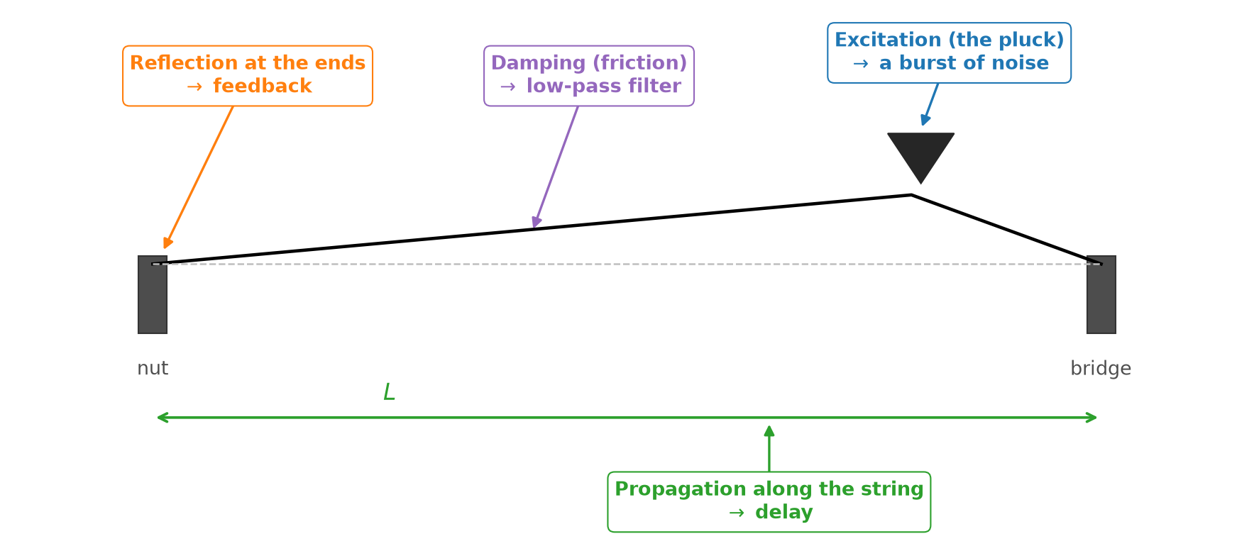
Fig. 84 A physical model of a plucked string. Each callout pairs a physical property of the string with the synthesis technique that simulates it.

Physical property	Simulation
Waves take time to travel along the string	A delay line
Waves reflect at the ends of the string	Feedback
Friction damps the waves, especially at high frequencies	Attenuation and a low-pass filter
A pluck excites the string at many frequencies at once	A burst of noise

In the rest of this section, we build up this model one physical property at a time: (1) propagation and reflection, (2) damping, and (3) excitation. Together, they form a classic algorithm for synthesizing plucked strings, called Karplus-Strong.

Propagation via feedback delay

Waves take time to travel. To simulate this, we use one of the simplest filters imaginable, one that simply delays its input. A delay line of \(M\) samples outputs its input \(M\) samples later:

\[y[n] = x[n - M].\]

Recall from Chapter 9 that in signal-flow diagrams, we draw a delay of \(M\) samples as a block labeled \(z^{-M}\).

On a string, waves also reflect at the ends and keep traveling back and forth. To simulate this, we feed back the output of the delay line into its input, where it adds to any new input, just as the reflected waves superimpose on the string:

\[y[n] = x[n] + y[n - M].\]

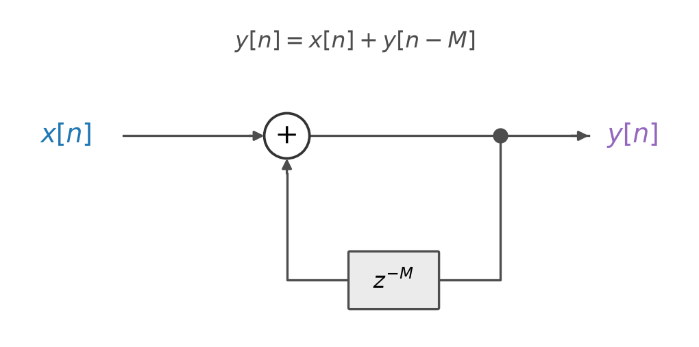
Fig. 85 A feedback delay line. The output \(y[n]\) is delayed by \(M\) samples and added back into the input.

Each trip around this loop simulates one round trip along the string, from the bridge to the nut and back. The wave reflects twice along the way, and each reflection inverts its polarity. So the wave returns with its original polarity, and the feedback simply adds it back in.

Delay lines as circular buffers

Why do we call it a delay line? To delay a signal by \(M\) samples, a filter must remember the last \(M\) samples that it has seen. We can picture them waiting in a line: at every time step, the newest sample joins the back of the line, and the oldest sample, from \(M\) samples ago, leaves at the front. In practice, we can implement a delay line as a data structure known as a circular buffer: an array of at least \(M\) samples, initialized with zeros, with a pointer to the oldest one. At each time step, we

1. read the oldest sample, \(y[n - M]\), at the pointer,

2. overwrite it with the newest sample, \(y[n]\), and

3. advance the pointer by one, wrapping around from the end of the array back to its start.

The animation below shows this in motion, for a feedback delay line with \(M = 3\). Each step reads the oldest sample at the gold pointer, adds the input, overwrites the oldest sample with the result, and advances the pointer. The pointer wraps around, but no sample ever moves, and the output repeats every \(3\) samples.

Each time step takes a constant amount of work, and the delay line takes a constant amount of memory, however long the signal. This makes circular buffers essential for real-time audio, which processes an endless stream of samples (Chapter 10).

The code below implements a feedback delay line with a circular buffer. Feeding it a short input reveals what makes it useful for physical modeling: whatever enters the loop comes back out every \(M\) samples, forever.

# hide
import numpy as np
import pyquist as pq

def feedback_delay(x: np.ndarray, M: int) -> np.ndarray:
    """A feedback delay line, y[n] = x[n] + y[n - M], stored in a circular buffer."""
    buffer = np.zeros(M)              # the delay line: the last M output samples
    i = 0                             # a pointer to the oldest one, y[n - M]
    y = np.zeros(len(x))
    for n in range(len(x)):
        y[n] = x[n] + buffer[i]       # 1. read y[n - M]
        buffer[i] = y[n]              # 2. overwrite it with y[n]
        i = (i + 1) % M               # 3. advance the pointer, wrapping around
    return y


x = np.array([1.0, 2.0, 3.0, 0.0, 0.0, 0.0, 0.0, 0.0, 0.0, 0.0, 0.0, 0.0])
print(feedback_delay(x, M=3))         # what enters the delay line returns every 3 samples

[1. 2. 3. 1. 2. 3. 1. 2. 3. 1. 2. 3.]

Tuning the delay line

How long should the delay line be? Suppose a wave travels \(L = 1\) meter at a speed of \(v = 400\) m/s. Working through the units, the delay in samples is

\[M \left[\text{samples}\right] = L \left[\text{meters}\right] \cdot \frac{1}{v} \left[\frac{\text{seconds}}{\text{meter}}\right] \cdot f_s \left[\frac{\text{samples}}{\text{second}}\right] = \frac{f_s \cdot L}{v}.\]

At \(f_s = 44{,}100\) Hz, our example wave takes \(M = 1 \cdot \frac{1}{400} \cdot 44{,}100 = 110.25\) samples. But a delay line can only delay by a whole number of samples, so we compromise by rounding: \(M = \mathrm{round}(\frac{f_s \cdot L}{v}) = 110\). Our simulated wave arrives a quarter of a sample early, as if it traveled about \(2\) mm less than it should. As we will see shortly, a shorter trip means a higher pitch.

How should we choose \(M\) to produce a particular fundamental frequency \(f\)? Recall that a string of length \(L\) has a fundamental frequency of \(f = \frac{v}{2L}\). Each trip around the loop covers a distance of \(2L\), so by the formula above, \(M = \frac{f_s \cdot 2L}{v}\). Substituting \(f = \frac{v}{2L}\),

\[M = \mathrm{round}\left(\frac{f_s}{f}\right).\]

The length of the delay line is simply the desired fundamental period, in samples. Notice that the length \(L\) and speed \(v\) of the string have dropped out entirely. To tune a feedback delay line, we only need the target frequency.

Rounding has a price, though. A feedback delay line can only produce the frequencies \(\frac{f_s}{M}\) for whole numbers \(M\). At low frequencies, \(M\) is large, and neighboring values of \(M\) produce nearly identical frequencies. For example, at \(f_s = 44{,}100\) Hz, \(M = 100\) produces \(441\) Hz and \(M = 101\) produces about \(436.6\) Hz, so we can tune to \(440\) Hz with an error of just \(1\) Hz. But at high frequencies, \(M\) is small, and the gaps between neighbors grow. For example, \(M = 11\) produces about \(4009\) Hz and \(M = 10\) produces \(4410\) Hz, a ratio of \(1.1\), or more than one and a half steps. The rounding error grows as frequency increases:

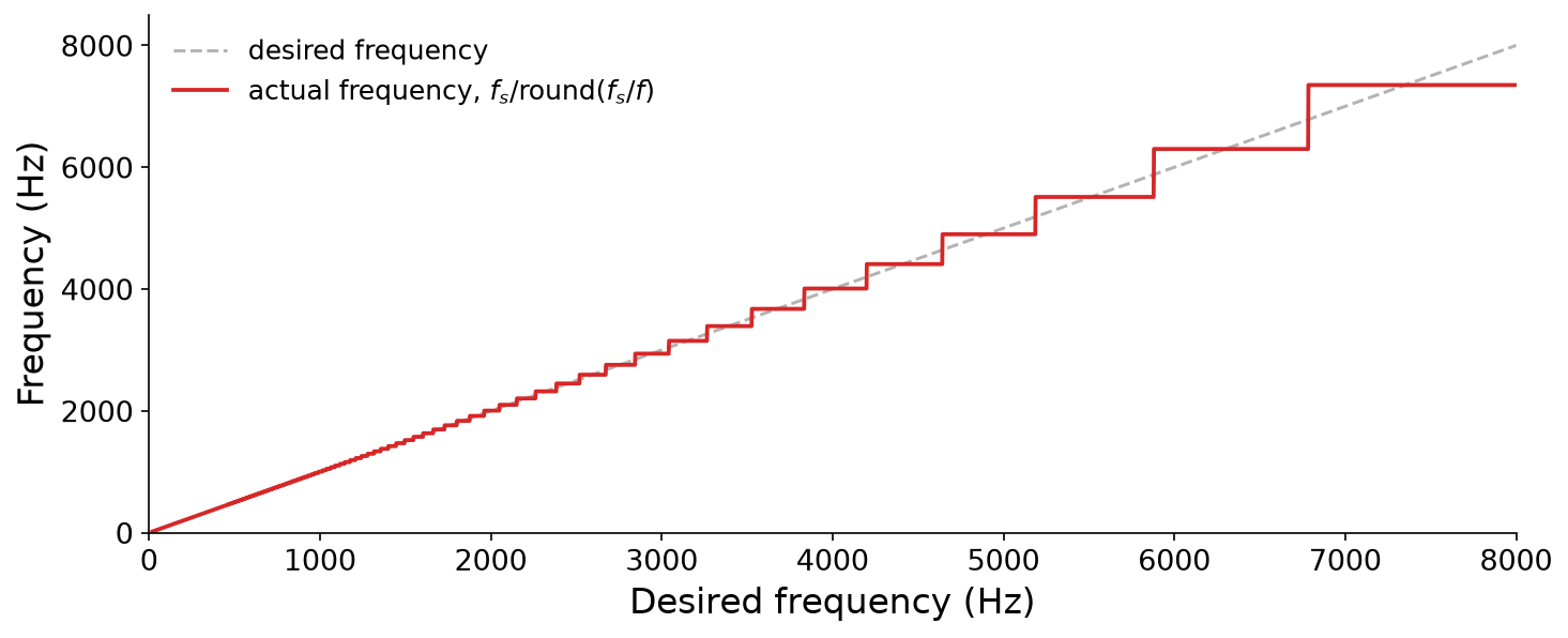
Fig. 86 The frequencies that a feedback delay line can produce at \(f_s = 44{,}100\) Hz when we round its delay to a whole number of samples (red), compared to the desired frequencies (dashed gray).

Another approach to tuning involves all-pass filters. Linear interpolation also acts as a low-pass filter, so inside a feedback loop, it changes how quickly the harmonics decay. Jaffe and Smith [JS83] instead used an all-pass filter, which leaves the amplitude of every frequency untouched, at the cost of a delay that is only exact at low frequencies.

Practical physical models avoid this problem with fractional delays, which delay a signal by a fraction of a sample. The simplest approach interpolates between neighboring samples, like the wavetables of Chapter 3. In this chapter, we will simply round.

Comb filters

Now, what does a feedback delay line do to a sound? It is a recursive filter, and therefore LTI, so recall from Chapter 9 that its impulse response tells us everything about it. Recall our feedback delay line, \(y[n] = x[n] + y[n - M]\). Its impulse response \(h\) is its output when the input is a unit impulse \(\delta = [1, 0, 0, \ldots]\), so \(h[n] = \delta[n] + h[n - M]\), where \(h[n] = 0\) for \(n < 0\). Let’s compute it one sample at a time:

\[\begin{split} \begin{aligned} h[0] &= \delta[0] + h[0 - M] &= 1 + 0 &= 1, \\ h[1] &= \delta[1] + h[1 - M] &= 0 + 0 &= 0, \\ &\;\;\vdots \\ h[M - 1] &= \delta[M - 1] + h[-1] &= 0 + 0 &= 0, \\ h[M] &= \delta[M] + h[0] &= 0 + 1 &= 1, \\ h[M + 1] &= \delta[M + 1] + h[1] &= 0 + 0 &= 0, \\ &\;\;\vdots \\ h[2M] &= \delta[2M] + h[M] &= 0 + 1 &= 1. \end{aligned} \end{split}\]

The impulse passes straight through at \(n = 0\), and then comes back out of the delay line every \(M\) samples:

\[\begin{split} h[n] = \begin{cases} 1 & \text{if } n = k \cdot M \text{ for some } k \in \mathbb{Z}_{\geq 0}, \\ 0 & \text{otherwise.} \end{cases} \end{split}\]

So the impulse response is an impulse train with a period of \(M\) samples, which never decays.

What is its frequency response? Recall from Chapter 7 that the spectrum of an impulse train is itself an impulse train. An impulse train with a period of \(M\) samples, or \(\frac{M}{f_s}\) seconds, has spikes in its spectrum every \(\frac{f_s}{M}\) Hz. So the feedback delay line boosts the frequencies at whole-number multiples of \(\frac{f_s}{M}\), and rejects the frequencies in between. Its magnitude response looks like the teeth of a comb, so it is called a comb filter:

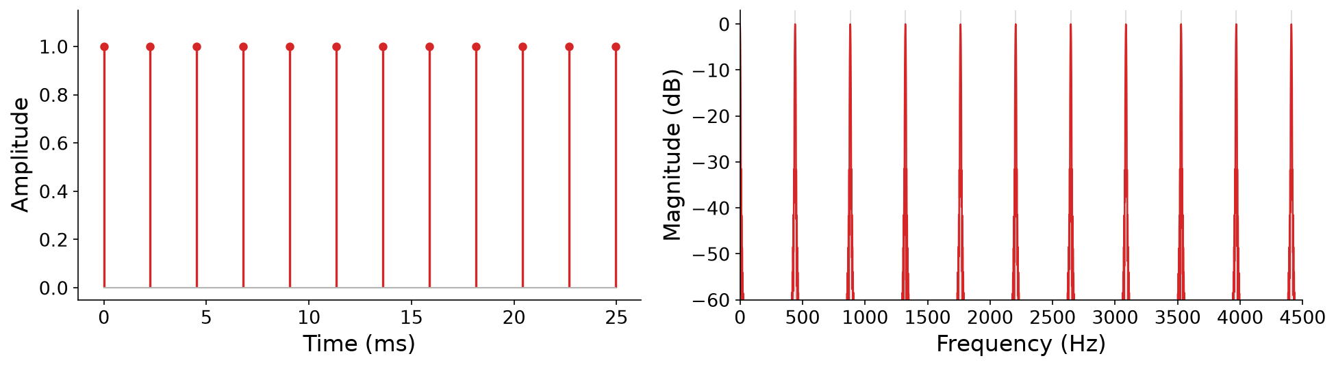
Fig. 87 The impulse response of a feedback delay line with \(M = 100\) at \(f_s = 44{,}100\) Hz (left) is an impulse train with a period of \(100\) samples, about \(2.27\) ms. Its spectrum (right, computed from the first \(0.25\) seconds of the impulse response) is a comb with teeth at multiples of \(\frac{f_s}{M} = 441\) Hz.

Aside from the tooth at \(0\) Hz, the teeth sit at \(\frac{f_s}{M}, \frac{2 f_s}{M}, \frac{3 f_s}{M}, \ldots\), which are exactly the harmonics of the fundamental frequency \(\frac{f_s}{M}\) that we tuned the delay line to. On its own, the frequency response of feedback delay emphasizes a fundamental frequency and its harmonics, just like a string.

The code below tunes our feedback delay line to \(220\) Hz and feeds it a unit impulse. It plots the first \(30\) ms of the impulse response, an impulse train, and the spectrum of the impulse response, a comb. Listen for a buzzy, sustained tone at \(220.5\) Hz, the closest frequency to \(220\) Hz that a whole number of samples allows:

# hide
import numpy as np
import pyquist as pq
from pyquist.helper import pitch_name_to_pitch, pitch_to_frequency

Show setup

Hide setup

# collapse
def feedback_delay(x: np.ndarray, M: int) -> np.ndarray:
    """A feedback delay line, y[n] = x[n] + y[n - M], stored in a circular buffer."""
    buffer = np.zeros(M)              # the delay line: the last M output samples
    i = 0                             # a pointer to the oldest one, y[n - M]
    y = np.zeros(len(x))
    for n in range(len(x)):
        y[n] = x[n] + buffer[i]       # 1. read y[n - M]
        buffer[i] = y[n]              # 2. overwrite it with y[n]
        i = (i + 1) % M               # 3. advance the pointer, wrapping around
    return y

f_s = 44100
M = round(f_s / 220.0)                    # tune the delay line to 220 Hz
impulse = np.zeros(f_s)                   # one second: a single 1, then zeros
impulse[0] = 1.0
h = pq.Audio(feedback_delay(impulse, M), f_s)
print(f"M = {M} audio samples, so the comb's teeth are {f_s / M:.2f} Hz apart")
pq.plot(h, duration=0.03)                                     # an impulse train...
pq.plot_freq(h, log_frequency=False).set_xlim(0, 2000)        # ...whose spectrum is a comb
pq.play(h)

M = 200 audio samples, so the comb's teeth are 220.50 Hz apart

From a single impulse, the feedback delay line produced a sustained, pitched tone with a harmonic spectrum. But unlike a real string, the tone never decays.

Damping via filters

Real strings don’t vibrate forever. On every trip along the string, a wave loses a little energy: to friction with the air, to friction inside the string, and to the body of the instrument, which radiates it as sound. Our feedback delay line, \(y[n] = x[n] + y[n - M]\), loses no energy at all. For example, with \(M = 2\), its impulse response is \(h = [1, 0, 1, 0, 1, 0, \ldots]\), which never decays.

Attenuation

To simulate this loss of energy, we attenuate the signal on every trip around the loop, by multiplying it by a gain \(0 < g < 1\). This gives the general form of a comb filter:

Definition 35 (Feedback comb filter)

A feedback comb filter with a delay of \(M \in \mathbb{Z}_{>0}\) samples and a gain \(g\) is the recursive filter

\[y[n] = x[n] + g \cdot y[n - M].\]

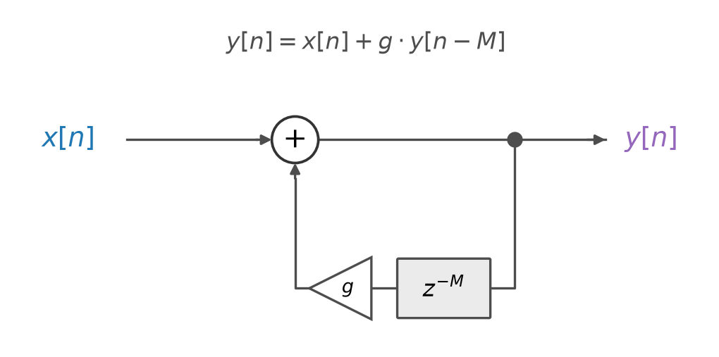
Fig. 88 A feedback delay line with attenuation. On every trip around the loop, the signal is multiplied by a gain \(g\).

Now, with \(M = 2\), the impulse response is \(h = [1, 0, g, 0, g^2, 0, g^3, \ldots]\). In general, for any delay \(M\), the impulse response is an impulse train that decays by a factor of \(g\) every \(M\) samples:

\[\begin{split}h[n] = \begin{cases} g^{n / M} & \text{if } n = k \cdot M \text{ for some } k \in \mathbb{Z}_{\geq 0}, \\ 0 & \text{otherwise.} \end{cases}\end{split}\]

As we saw in Chapter 9, this filter is stable for \(|g| < 1\), and its impulse response decays exponentially. In the frequency domain, the teeth of the comb stay at whole-number multiples of \(\frac{f_s}{M}\), but the smaller the gain \(g\), the wider and shallower they become:

Fig. 89 With attenuation, the impulse response of a feedback delay line decays exponentially (left, with \(M = 100\) and \(g = 0.8\)). Its spectrum is still a comb with teeth at multiples of \(\frac{f_s}{M} = 441\) Hz, but the teeth widen as \(g\) decreases (right).

Setting the decay time

How should we choose \(g\)? Musically, we want to control the duration of a note independently of its pitch. But the duration depends on both \(g\) and \(M\), because the signal is attenuated once per trip around the loop, and the number of trips per second depends on \(M\).

Technically, an exponentially decaying impulse response only reaches zero in the limit as \(t \to \infty\). But in practice, it becomes inaudible long before then. As in Chapter 9, we could consider a sound to be “over” once it has decayed by \(60\) dB, to \(10^{-60/20} = 10^{-3}\) of its initial amplitude. So what gain \(g\) makes the impulse response decay by \(60\) dB in \(T\) seconds?

After \(k\) trips around the loop, the peak amplitude of the impulse response is \(g^k\). Working through the units, the number of trips in \(T\) seconds is

\[k \left[\text{trips}\right] = T \left[\text{seconds}\right] \cdot f_s \left[\frac{\text{samples}}{\text{second}}\right] \cdot \frac{1}{M} \left[\frac{\text{trips}}{\text{sample}}\right] = \frac{f_s T}{M}.\]

Setting the amplitude after these \(k\) trips to \(10^{-3}\) and solving for \(g\),

\[g^{f_s T / M} = 10^{-3} \quad \Longrightarrow \quad \frac{f_s T}{M} \cdot \log_{10} g = -3 \quad \Longrightarrow \quad g = 10^{-3M / (f_s T)}.\]

Notice that \(g\) depends on both the duration \(T\) and the pitch, via \(M\). For example, at \(f_s = 44{,}100\) Hz, a note at \(220.5\) Hz has \(M = 200\), so it makes \(\frac{44{,}100}{200} = 220.5\) trips per second. To decay by \(60\) dB in \(T = 1\) second, it needs \(g = 10^{-3/220.5} \approx 0.969\). A note an octave higher makes twice as many trips per second, so to last just as long, it needs a gain closer to \(1\), \(g = 10^{-3/441} \approx 0.984\).

The code below puts this to use in an instrument, pluck_like(pitch, duration), which tunes a damped feedback delay line to a pitch, computes \(g\) from the duration, and excites the delay line with a unit impulse. We use it to render a short sequence of notes with a pq.Score, as in Chapter 4:

# hide
import numpy as np
import pyquist as pq
from pyquist.helper import pitch_name_to_pitch, pitch_to_frequency

def feedback_delay(x: np.ndarray, M: int, g: float = 1.0) -> np.ndarray:
    """A feedback delay line with attenuation, y[n] = x[n] + g * y[n - M]."""
    buffer = np.zeros(M)              # the delay line, as a circular buffer
    i = 0
    y = np.zeros(len(x))
    for n in range(len(x)):
        y[n] = x[n] + g * buffer[i]   # attenuate y[n - M] on every trip
        buffer[i] = y[n]
        i = (i + 1) % M
    return y


def pluck_like(pitch: str, duration: float, f_s: int = 44100) -> pq.Audio:
    """An impulse through a damped feedback delay line that decays by 60 dB over `duration`."""
    M = round(f_s / pitch_to_frequency(pitch_name_to_pitch(pitch)))
    g = 10 ** (-3 * M / (f_s * duration))
    impulse = np.zeros(int(duration * f_s))
    impulse[0] = 1.0
    return pq.Audio(feedback_delay(impulse, M, g), f_s)


melody = pq.Score([(0.0, {"pitch": "C4", "duration": 2.0}),
                   (0.5, {"pitch": "E4", "duration": 2.0}),
                   (1.0, {"pitch": "G4", "duration": 2.0}),
                   (1.5, {"pitch": "C5", "duration": 4.0})])
pq.play(melody.render(pluck_like), normalize=True)

The notes now decay like plucked strings. But they still sound buzzy and artificial, more like a toy than a guitar.

Low-pass filtering

Why? Multiplying by \(g\) is, technically, a filter, \(y[n] = g \cdot x[n]\). But it scales every frequency by the same amount, so all of the harmonics decay at the same rate. In a real string, the higher harmonics decay much faster than the lower ones, so a plucked note starts bright and then mellows as it rings.

To simulate this, we add a low-pass filter to the loop, which attenuates the higher frequencies more on every trip. The simplest low-pass filter of all is a two-point average, \(\frac{1}{2}(x[n] + x[n - 1])\), which is the first filter that we studied in Chapter 9, scaled by \(\frac{1}{2}\). Placing it in the loop,

\[y[n] = x[n] + g \cdot \tfrac{1}{2}\big(y[n - M] + y[n - M - 1]\big).\]

Now, the higher the frequency of a harmonic, the more it is attenuated on every trip. So the high harmonics die away quickly, while the low harmonics ring on:

Gain only

Gain and low-pass

Spectrograms of a damped feedback delay line tuned to \(110\) Hz and excited by a unit impulse, with a gain alone (left) and with a gain and a two-point average (right). With the low-pass filter in the loop, the higher harmonics decay faster, and the pluck sounds more natural.

We will put this low-pass filter into code shortly, along with the final ingredient of our physical model.

Excitation via noise

So far, we have excited our physical model with a unit impulse. Is this a good model of a pluck? During the first \(M\) samples, the feedback path contributes nothing, so the output is just the input. In effect, the first \(M\) samples of the input fill the delay line with an initial waveform, which the loop then recirculates, attenuating and smoothing it on every trip.

What should this initial waveform be? A pluck, a strike, or the scrape of a bow is a sudden, chaotic event, which excites an instrument at many frequencies at once. So the sounds of instruments typically start out noisy and broadband, and then become periodic and resonant. This suggests filling the delay line with noise. We have casually used noise as a sound source in previous chapters, like in the subtractive synthesis of Chapter 9. Let’s now define white noise formally.

Definition 36 (White noise)

A random signal \(x[n]\) is white noise if its samples are independent and identically distributed, with mean zero.

In this book, we draw each sample of white noise uniformly at random between \(-1\) and \(1\). Just as white light contains all visible colors in roughly equal measure, white noise contains all frequencies in equal measure. Any one spectrum of white noise is jagged, since every frequency bin is random, but on average, it is flat:

Fig. 90 Ten milliseconds of white noise, with samples drawn uniformly between \(-1\) and \(1\) (left), and the magnitude spectrum of one second of it (right). Each bin of the spectrum is random (light blue), but on average (black), the spectrum is flat from \(0\) Hz up to the Nyquist frequency.

To simulate a pluck, we excite the delay line with one period of white noise: \(x[n]\) is white noise for \(0 \leq n < M\), and \(x[n] = 0\) for \(n \geq M\). White noise contains all frequencies, so it excites every harmonic at once. The loop then recirculates the noise once per period, so the output is pitched right away. On every trip, the low-pass filter smooths the noise a little more, so the sound starts bright and noisy, like the attack of a pluck, and mellows as it decays.

An impulse also contains all frequencies, so why does noise make a better pluck? An impulse excites every harmonic with exactly the same amplitude and phase, which sounds thin and buzzy. Noise excites each harmonic with a random amplitude and phase, which sounds richer and more natural, and makes every pluck slightly different, just like on a real instrument:

Excited by a unit impulse

Excited by a burst of white noise

The same feedback delay line, with a gain and a two-point average in its loop, tuned to \(196\) Hz and decaying by \(60\) dB over \(2.5\) seconds. It is excited by a unit impulse (first) and by one period of white noise (second).

The Karplus-Strong algorithm

Putting all of these pieces together yields one of the most famous algorithms in computer music, the Karplus-Strong algorithm, published by Kevin Karplus and Alex Strong in 1983 [KS83]:

Fig. 91 The Karplus-Strong algorithm. A burst of noise excites a feedback delay line, with a low-pass filter and attenuation in its loop.

Definition 37 (Karplus-Strong algorithm)

The Karplus-Strong algorithm synthesizes a plucked string with fundamental frequency \(f\), lasting \(T\) seconds at sample rate \(f_s\), by computing

\[y[n] = x[n] + g \cdot \tfrac{1}{2}\big(y[n - M] + y[n - M - 1]\big),\]

where

1. the delay \(M = \mathrm{round}\big(\frac{f_s}{f}\big)\) tunes the loop,

2. the gain \(g = 10^{-3M / (f_s T)}\) decays the output by about \(60\) dB in \(T\) seconds, and

3. the excitation \(x[n]\) is white noise for \(0 \leq n < M\), and zero otherwise.

Karplus and Strong’s original algorithm had no gain, i.e., \(g = 1\). Its notes still decay, because of the low-pass filter. In fact, higher notes decay faster, because they make more trips around the loop per second, just like on real strings. David Jaffe and Julius Smith later proposed several extensions to the algorithm [JS83], including ways to control its decay time, like our gain \(g\).

Karplus and Strong originally described their algorithm as a variation on the wavetable synthesis of Chapter 3. The delay line is a wavetable of \(M\) samples, initialized with random values, which the algorithm reads in a loop, smoothing the table a little on every pass.

The code below implements the Karplus-Strong algorithm as an instrument, karplus_strong(pitch, duration). Its delay line is a circular buffer, and its low-pass filter keeps a memory of its own: the previous sample to leave the delay line. We use it to strum all six strings of a simulated guitar, one string every \(40\) ms. Run it a few times: since the excitation is random, every strum sounds slightly different.

# hide
import numpy as np
import pyquist as pq
from pyquist.helper import pitch_name_to_pitch, pitch_to_frequency

def karplus_strong(pitch: str, duration: float, f_s: int = 44100) -> pq.Audio:
    """A plucked string: a burst of white noise through a damped, low-passed feedback delay line."""
    M = round(f_s / pitch_to_frequency(pitch_name_to_pitch(pitch)))
    g = 10 ** (-3 * M / (f_s * duration))      # decay by about 60 dB over the duration
    N = int(duration * f_s)
    x = np.zeros(N)
    x[:M] = np.random.uniform(-1.0, 1.0, M)    # excitation: one period of white noise
    buffer = np.zeros(M)                       # the delay line, as a circular buffer
    i = 0
    previous = 0.0                             # the low-pass filter's memory, y[n - M - 1]
    y = np.zeros(N)
    for n in range(N):
        delayed = buffer[i]                                  # y[n - M]
        y[n] = x[n] + g * 0.5 * (delayed + previous)         # low-pass, attenuate, and add
        previous = delayed
        buffer[i] = y[n]
        i = (i + 1) % M
    return pq.Audio(y, f_s)


# Strum all six strings of a guitar (an E minor chord), one string every 40 ms
strum = pq.Score([(0.04 * i, {"pitch": pitch, "duration": 3.0})
                  for i, pitch in enumerate(["E2", "B2", "E3", "G3", "B3", "E4"])])
pq.play(strum.render(karplus_strong), normalize=True)

With just a few lines of code, and a handful of arithmetic operations per audio sample, we have synthesized a convincing plucked string.