import matplotlib
if not hasattr(matplotlib.RcParams, "_get"):
matplotlib.RcParams._get = dict.get
16.1 Music generation#
How did we get from algorithmic composition techniques like Markov chains (Chapter 14) to modern music generation systems like Suno? In this section, we will trace a few of the key ideas, first for generating symbolic music (scores), and then for generating audio.
From n-grams to neural language models#
Recall from Chapter 14 that an \(n\)-gram model predicts each note from the \(n - 1\) notes before it:
where the probabilities are computed by counting \(n\)-grams in the training data. A model of this form, which assigns probabilities to sequences by predicting each element from the elements before it, is often called a language model (LM). The term comes from natural language, where the elements are words, but the same idea applies to notes:
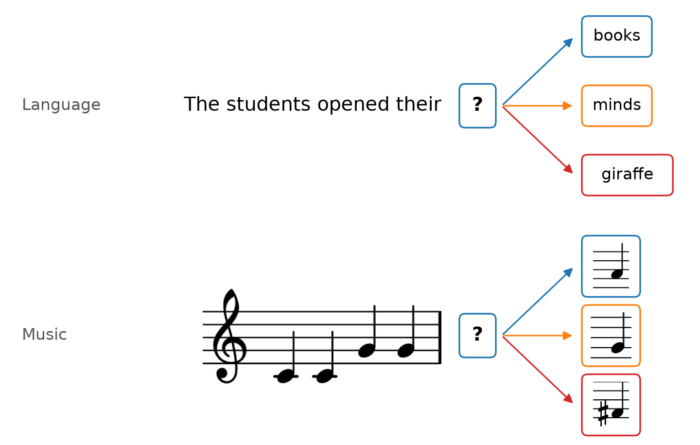
Fig. 132 Language models predict the next element of a sequence from the elements before it, whether the elements are words (top) or notes (bottom). A good language model assigns high probabilities to likely continuations (blue) and low probabilities to unlikely ones (red).#
The key issue with \(n\)-gram models is the curse of dimensionality. An \(n\)-gram model over an alphabet \(\mathcal{X}\) has \(|\mathcal{X}|^n\) probabilities. This blows up in memory, and it also blows up in sparsity, since most of the possible \(n\)-grams never appear in the training data. To see why sparsity is such a problem, consider an example with words.
Example 5 (Sparse counts)
Consider a tiny dataset of three sentences:
rabbits are fast. cheetahs are quick. turtles are slow.
How likely are the new sentences “rabbits are quick” and “turtles are quick”? Here are the probabilities of the word “quick” that bigram and trigram models count from the dataset:
Model |
Rabbits are quick |
Turtles are quick |
|---|---|---|
Bigram |
\(P(\text{quick} \mid \text{are}) = \frac{1}{3}\) |
\(P(\text{quick} \mid \text{are}) = \frac{1}{3}\) |
Trigram |
\(P(\text{quick} \mid \text{rabbits are}) = 0\) |
\(P(\text{quick} \mid \text{turtles are}) = 0\) |
The bigram model can’t tell the two sentences apart. Its context is too short to capture their meaning. The trigram model’s context is long enough, but it has never seen either trigram, so both sentences get a probability of \(0\). Its counts are too sparse.
With a short context, an \(n\)-gram model can’t capture meaning. With a long context, it needs exponentially more data. How do we reconcile this tension? The key insight of neural language models is to use a distributed representation, in which similar elements and contexts are represented similarly [BDVJ03]. If a model could somehow learn that rabbits and cheetahs are both fast animals, and that “fast” and “quick” mean similar things, it could generalize from “cheetahs are quick” to “rabbits are quick”, without ever seeing that particular trigram.
Neural language models also aim to take into account far more context than \(n\)-gram models, possibly up to the entire history of the sequence. In its most general form, a neural language model conditions each element on all of the elements before it:
Definition 53 (Neural language model)
A neural language model is a neural network \(f_\theta\), with parameters \(\theta\), that maps the elements of a sequence so far to a probability distribution over the next element:
Notice that this has the same “type signature” as an \(n\)-gram model. Both are functions that take a context as input and output an array of probabilities (that sum to \(1\)), one for each element of the alphabet. For an \(n\)-gram model, \(f : \mathcal{X}^{n-1} \to [0, 1]^{|\mathcal{X}|}\) is a lookup table of counted probabilities. For a neural language model, \(f_\theta : \mathcal{X}^* \to [0, 1]^{|\mathcal{X}|}\) is a neural network that accepts contexts of any length (\(\mathcal{X}^*\) denotes the set of sequences of any length).
A neural network is a long chain of simple arithmetic operations, whose behavior is determined by its parameters \(\theta\), a large set of real numbers. The details of neural networks are out of scope for this book. For the purposes of this textbook, we will treat \(f_\theta\) as a black box.
The key is the number of parameters. For example, with an alphabet of \(16\) pitches, a \(5\)-gram model has \(16^5 \approx 1\) million probabilities, most of which are zero for lack of data. A simple neural language model may have as few as a few thousand parameters, so \(|\theta| \ll |\mathcal{X}|^n\). Since there are far fewer parameters than possible contexts, the network must share information between similar contexts, which is exactly what \(n\)-gram models fail to do.
Training#
How do we set the parameters \(\theta\)? In Chapter 14, we chose \(n\)-gram probabilities to maximize the likelihood of the training data, and it turned out that counting does exactly that. For a neural network, the goal is the same, but there is no closed form solution for the optimal parameters.
Instead, we define a loss function that measures how poorly the model fits the training data, and search for the parameters that minimize it:
Definition 54 (Training a language model)
Given a training sequence \(x_1, \ldots, x_N\), training minimizes the average negative log-likelihood,
Minimizing this loss is the same as maximizing the likelihood of the training data.
This may look familiar. Recall the definition of entropy from Chapter 15, \(H(X) = -\sum_{x} P(x) \log P(x)\). In the training data, the actual next element \(x_i\) is known, so we can treat its probability as \(P(x_i) = 1\), and the probability of every other element as \(0\). If we use the model’s probabilities inside the logarithm, only one term of the sum remains, \(-\log P_\theta(x_i \mid x_1, \ldots, x_{i-1})\), and the loss is just its average. In other words, the loss is essentially the entropy of the training data, as measured by the model (technically, the cross-entropy). With a base-\(2\) logarithm, it is measured in bits per element, so a better language model is also a better compressor.
We minimize the loss with gradient descent: starting from random parameters, we repeatedly compute the gradient of the loss with respect to the parameters, \(\nabla_\theta \mathcal{L}\), and take a small step downhill, \(\theta \leftarrow \theta - \eta \nabla_\theta \mathcal{L}\), where \(\eta\) is the learning rate. The gradient can be computed efficiently with an algorithm called backpropagation. Intuitively, each step nudges the predicted probabilities closer to the actual next notes:
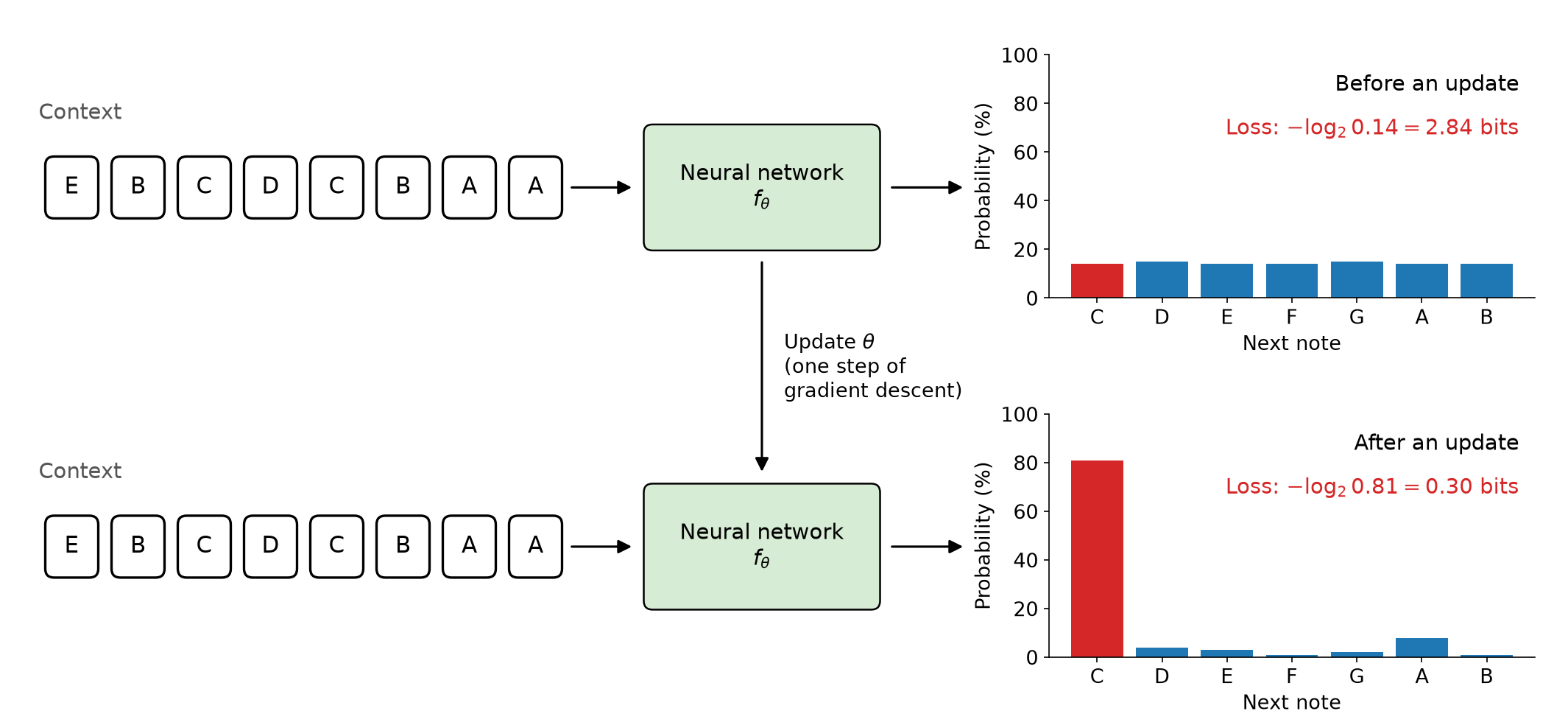
Fig. 133 A neural language model’s predictions for the note after the context E B C D C B A A, whose actual next note is C (red), before (top) and after (bottom) an update of its parameters \(\theta\). The update lowers the loss for this example from \(2.84\) to \(0.30\) bits. Training repeats such updates for many examples.#
More expression, context, and data#
Along with moving from simple \(n\)-gram statistics to neural models, music language models have improved in three other important dimensions.
More expression. To fight the curse of dimensionality, \(n\)-gram models kept their alphabets small, for example, the \(12\) pitch classes. This sacrificed a lot of nuance. With neural models, we can afford larger alphabets (often called vocabularies) that capture more of the music:
Alphabet |
Size |
Twinkle, Twinkle, Little Star |
|---|---|---|
Pitch classes |
\(12\) |
C, C, G, G, A, A, G |
+ octaves |
\(88\) (piano keys) |
C4, C4, G4, G4, A4, A4, G4 |
+ durations |
\(88 \cdot 2\) (with two note lengths) |
♩C4, ♩C4, ♩G4, ♩G4, ♩A4, ♩A4, ♩♩G4 |
To represent polyphony, Performance RNN [OSD+20] encoded music as a sequence of events, much like MIDI (Chapter 15): “note on” and “note off” events for each pitch, and “time shift” events that advance time. For example, a C major chord followed by a melody note one beat later might be encoded as C3, E3, G3, C4, (shift 1 beat), G4. Additional “velocity” events set the loudness of the notes that follow, so the model can capture an expressive performance, not just a score.
More context. An \(n\)-gram model sees only a finite context of \(n - 1\) elements. The goal of a neural language model is to condition on the entire history of the sequence, no matter how long. Music has structure at long timescales, such as a chorus that returns minutes later, so the more context a model can use, the better. Today, most language models are based on the Transformer [VSP+17], a neural network that can look directly at each element of long contexts. The Music Transformer applied it to piano music [HVU+19].
More data. Finally, rather than fitting a model to a single song, modern models are trained on thousands or millions of songs.
Let’s put these ideas together. A lead sheet is a simple score of a popular song, consisting of its melody and its chords. The code below generates new lead sheets with a neural language model \(f_\theta\), trained ahead of time on about \(9{,}000\) lead sheets from the Hooktheory dataset [DTL22]. Each lead sheet is a sequence of tokens: melody notes, chord changes, time shifts, and bar lines. Just like with Markov chains, we generate one token at a time, by drawing each next token from the probabilities that the model predicts. For comparison, the code also generates a lead sheet with the same neural network before training, with random parameters \(\theta\):
MAX_TOKENS = 512 # stop here, even before 16 bars
def generate(f_theta: Callable[[list[int]], np.ndarray]) -> list[int]:
tokens = [INDEX["<BOS>"]] # the beginning of a song
while tokens.count(INDEX["BAR"]) <= 16 and len(tokens) < MAX_TOKENS: # 16 bars
p = f_theta(tokens) # P(next token | all tokens so far)
p[INDEX["<EOS>"]] = 0 # don't let the song end early
tokens.append(np.random.choice(len(VOCAB), p=p / p.sum()))
return tokens
for trained in [True, False]:
print("After training:" if trained else "Before training (random parameters):")
f_theta = load_model("./assets/lead-sheet-rnn.npz", trained=trained)
tokens = generate(f_theta)
print([VOCAB[token] for token in tokens[:12]], "...")
melody, chords = tokens_to_events(tokens)
pq.play(lead_sheet_to_score(melody, chords).render(band), normalize=True)
After training:
['<BOS>', 'BAR', 'CHORD_G#:maj', 'SHIFT_4', 'NOTE_63', 'SHIFT_4', 'NOTE_60', 'SHIFT_2', 'NOTE_63', 'SHIFT_4', 'NOTE_61', 'BAR'] ...
Before training (random parameters):
['<BOS>', 'CHORD_F:7', 'NOTE_79', 'CHORD_C:min', 'SHIFT_9', 'CHORD_D:min7', 'CHORD_E:maj', 'NOTE_78', 'CHORD_B:7', 'CHORD_F:min', 'BAR', 'NOTE_80'] ...
Before training, the model’s predictions are nearly uniform, so it produces a jumble of random notes and chords. After training, the generated lead sheets have plausible local statistics. For example, most of their melody notes belong to the chord being played, just as in real songs. But they rarely repeat a bar, while real pop songs repeat bars all the time. Long-term structure remains a challenge. If you want to learn more, this notebook shows how the model (a small recurrent neural network) was trained, using the PyTorch library.
n-grams vs. modern language models#
Compared to the \(n\)-gram models of Chapter 14, modern music language models differ in their context, their alphabet, their model, and their training:
\(n\)-gram model |
Modern music LM |
|
|---|---|---|
Context |
The previous \(n-1\) elements |
Up to the entire history |
Alphabet |
Pitch classes |
Events with octaves, durations, polyphony, and expression |
Model |
A lookup table of \(|\mathcal{X}|^n\) probabilities |
A neural network \(f_\theta\) with parameters \(\theta\) |
Training |
Counting \(n\)-grams statistics for a few pieces |
Gradient descent on thousands or millions of pieces |
Despite these differences, they share many similarities! Both are language models with the same type signature, \(P(\text{next} \mid \text{context})\), and both generate music the same way, by drawing one element at a time.
Generating audio#
Scores are great, but how do we generate audio? What if we simply trained a language model on audio samples? This is exactly the idea of WaveNet [vdODZ+16], which predicts each sample of a waveform from the samples before it:
To make this a language model over a finite alphabet, WaveNet quantizes each sample to one of \(256\) values. Recall that Chapter 14 also predicted each sample from the previous ones, with linear predictive coding. WaveNet takes the same idea and increases the size of the model (a deep neural network instead of a linear filter), the amount of training data, and the context, much like the path from \(n\)-grams to modern music language models. To see thousands of samples of context, WaveNet stacks dilated causal convolutions, layers of filters (Chapter 9) that each look further into the past than the one before:

Fig. 134 WaveNet’s stack of dilated causal convolutions. Each layer combines two values from the layer below, which are farther apart in each successive layer (the dilation doubles). The rightmost output (orange) depends on all \(16\) input samples (red paths), even though each layer only combines two values. An animated version appears in DeepMind’s original blog post.#
WaveNet is capable of generating remarkably realistic audio, sample by sample. Here are two examples from a very large WaveNet trained on piano music, at a sample rate of \(16\) kHz [DvdOS18]:
Piano music generated sample by sample by a very large WaveNet, from Dieleman et al. (2018).
The timbre of the piano is convincing, but the music sounds like it’s just wandering aimlessly. Why might this be the case?
Codec language models#
The trouble is that waveforms are long. At \(44.1\) kHz, a three-minute stereo pop song has about \(16\) million samples, far longer than the sequences that language models typically handle:
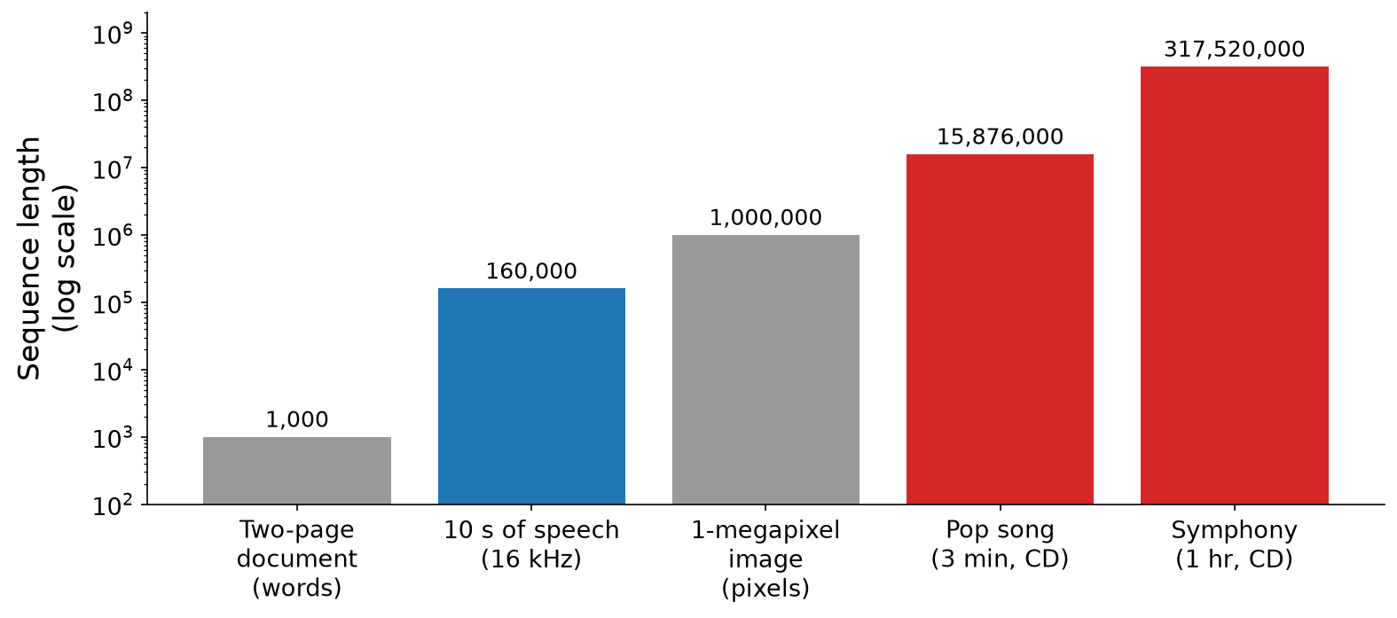
Fig. 135 Sequence lengths in perspective (log scale). Audio waveforms (red) are orders of magnitude longer than the documents that language models are typically trained on.#
Meanwhile, music has structure at many timescales. The period of a \(440\) Hz sinusoid is about \(2\) ms, and the attack of a note is about \(10\) ms. At \(120\) BPM, a beat lasts \(500\) ms and a measure \(2\) s. A pop chorus lasts about \(20\) s, a pop song about \(3\) minutes, and a symphony about an hour. That’s more than six orders of magnitude! A model that sees thousands of samples of context, like WaveNet, captures only the shortest of these timescales.
How can we model such long sequences? Recall from Chapter 15 that much of the detail in a waveform is irrelevant to human perception. Perhaps we can compress the audio first! But rather than designing a codec by hand, like MP3, we can learn one from data. A codec language model works in three stages [DJP+20, DvdOS18, vdOVK17]:
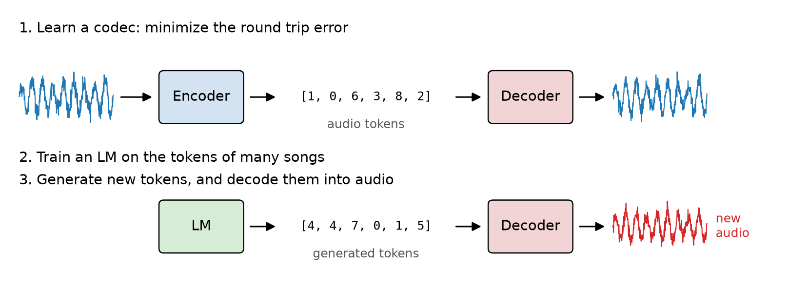
Fig. 136 A codec language model. (1) An encoder and a decoder, both neural networks, are trained together to minimize the error of the round trip from audio to discrete tokens and back. (2) A language model is trained on the tokens of many songs. (3) To generate audio, the language model generates new tokens, and the decoder turns them into audio.#
In the terminology of Chapter 15, the encoder is a learned coder, and the decoder is a learned decoder. The codes are discrete tokens from a finite alphabet, at a rate two to three orders of magnitude lower than the sample rate, which makes the sequences short enough for a language model. Listen to the difference between the WaveNet samples above and samples from a codec language model of piano music, from the same paper:
Control#
How do we control these models? If we have training examples of pairs of (control, music), we can simply put the control information in the context, before the music. The model learns to predict music that fits the control. To generate, we choose the control ourselves, and let the model generate the rest:
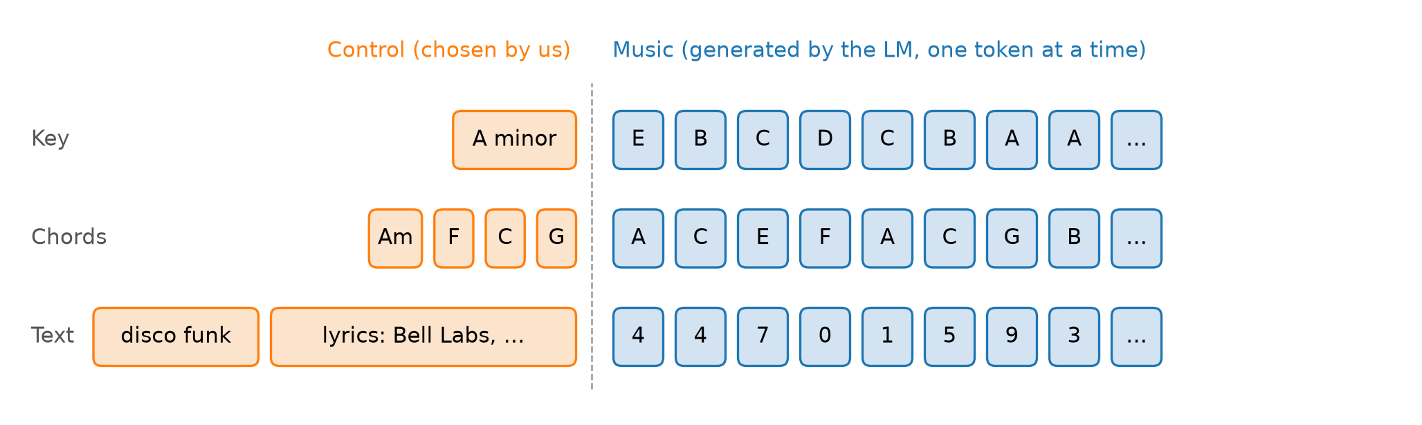
Fig. 137 Controlling a language model. Each training sequence begins with control tokens, such as a key (top), chords (middle), or a text description and lyrics (bottom), followed by the music. To generate, we choose the control tokens, and the model generates the music tokens that follow.#
Jukebox [DJP+20] combined these ideas: a codec language model, trained on a large collection of popular music recordings, and controlled by the genre, the artist, and the lyrics. It was one of the first models to generate music audio in a broad range of styles, complete with singing:
Jukebox: jazz, in the style of Ella Fitzgerald
Jukebox: classic pop, in the style of Frank Sinatra
Two samples from OpenAI’s Jukebox (2020), conditioned on a genre, an artist, and lyrics.
Jukebox also brought ethical and legal questions to the forefront. It was trained on large volumes of copyrighted music, likely without the consent of the musicians who created it, and can imitate the styles and voices of specific artists. We will return to these questions at the end of this chapter, along with modern approaches to controlling music generation with text.
Beyond language models#
There are other ways to train music generation models besides language models. Diffusion models [HJA20] learn to gradually remove noise from data. To generate, they start from pure noise and denoise it step by step. Many modern music generation systems combine a diffusion model with a learned autoencoder, which compresses audio much like a codec, but into continuous values rather than discrete tokens [ECT+24]. Before diffusion models, generative adversarial networks (GANs) [GPAM+14], which pit a generator network against a discriminator network, were a popular approach to audio generation [DMP19, EAC+19]. We won’t cover these approaches here, but these papers are good places to start.