Detailed Research Interests
1.0 Constrained Motion Planning
Mobile robots, at least wheeled ones,
are trickier than manipulators in
many fundamental ways. First, they are described adequately only by
differential equations - rather than kinematic ones. Second, those
kinematic equations are subject to constraints - its constrained
dynamics. Third, those constraints are "nonholonomic" meaning they
cannot be integrated (not all equations can be integrated in closed
form). Fourth, the constraints are not satisfied as soon as the wheels
begin to slip and characterizing slip is even harder! Motion planning
for mobile robots is a search problem in the continuum of path space
subject to differential constraints. You figure that stuff out every
time you park your car.
1.1 Lattice Planner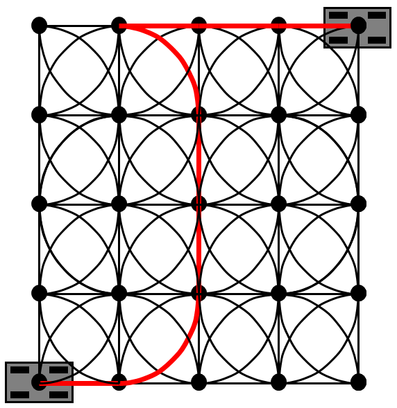
The development of the lattice planner
[pdf] concept is really an effort in
search space design rather than motion planning. By exploiting our general
trajectory generatordescribed
below, we are able to construct search spaces for
motion planning which are inherently feasible - meaning the robot
can execute the paths encoded in the lattice directly. The lattice
is a regular array of states in state space - each of which is joined
to its local neighbors by a repeating arrangement of dynamically
feasible edges. This type
of planner is perfect for wheeled
mobile robots because their nonholonomic constraints are satisfied by
default in the search space, so planning becomes simply a search
process - with no constraints to worry about. Intricate multi point
turns in very dense obstacle fields
become easy to generate with this approach. The image opposite shows a
lattice for the Reeds-Shepp car showing one maneuver that is encoded in
the
space.
Click the image opposite
to see a mars rover navigate its way home using the lattice planner.
The lattice planner was the basis of the parking lot planner used on
the Darpa Urban Challenge.
Pivtoraiko, M., Kelly, A., Knepper, R., “Differentially Constrained Mobile Robot Motion
Planning in State Lattices”, Journal of Field Robotics, Volume 26 , Issue 3, (March 2009),
pp 308-333. [pdf]
1.2 Trajectory Generator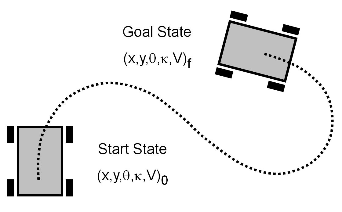
Our work in trajectory generation
[pdf]
has,
after several iterations and refinements resulted in a general approach
to the problem of inverting the dynamics of any vehicle. By
expressing arbitrary controls in terms of the Taylor series
coefficients, we are able to convert the intrinsic optimal control
problem into an equivalent constrained optimization problem. In
practice, coupled with numerical linearization techniques, this means we can invert a model of any vehicle on arbitrary
terrain given a predictive model of actuator response, delays, body
dynamics, and wheel terrain interactions, etc. Getting such a model is
a problem in itself which is discussed below in the
calibration section.
The figure motivates the problem for a car that needs to move far
right, slightly forward and turn 90 degrees counterclockwise.
Click the image to see
a mars rover compensate predictively for the yaw moment caused by a
stuck rear wheel. Since the trajectory generator can invert any model,
this system can even invert a model that is being adapted based on
experience.
Howard, T., Kelly, A., “Optimal Rough Terrain Trajectory Generation for Wheeled Mobile
Robots”, The International Journal of Robotics Research, Vol. 26, No. 2, pp. 141-166 (Feb
2007). [pdf].
2.0 Advanced Controls
Controls for mobile robots are
complicated by the same issues as in motion planning. The
underactuation that tends to go hand-in-hand with nonholonomic
constraints means that merely responding to the present errors is not a
good approach. Mobile robot controls need to be predictive to prevent
errors before they occur since there may be no way to actuate them away
easily afterwards.
2.1 Urban Challenge Lane Following Controller

The
trajectory generator was the
basis of the lane following controller used on the
Darpa Urban Challenge. Here, we use its capacity to generate a smooth
trajectory anywhere in order to generate continuous paths which terminate
precisely lined up with arbitrary lane geometry while spanning the
lane. These planning options can be used to change lanes or avoid
obstacles in a very natural manner.
Click the image to
see this controller first in simulation. Then watch it avoid a collision
with the dreaded giant "Terramax" vehicle in the Urban Challenge. It would have been a very bad day for robots otherwise.
Howard, T., Green, C., Kelly, A.,Ferguson, D. “State Space
Sampling of Feasible Motions for High Performance Mobile Robot
Navigation in Complex Environments”, Journal of Field Robotics.
Vol 25, No 6-7 June 2008, pp. 325-345. [pdf].
2.2 Receding Horizon Path Following
Such
a trajectory generator concept
can also be applied to forms of optimal
control including model predictive control. Here we use the same
parameterization concept but apply it to optimal control directly - by
minimizing the objective function. The
result is a controller that can follow arbitrarily complicated
trajectories that exploit the full maneuverability envelope of the
platform. The system even predicts and compensates for error through
velocity reversals as shown in the the figure opposite. Here the vehicle
needs to turn around and exit the obstacle field in reverse. The
vehicle has significant crosstrack error but the recovery control gets
it rapidly back on the desired.state space trajectory.
T. Howard, C. Green, A. Kelly, “Receding Horizon Model-Predictive
Control for Mobile Robot Navigation of Intricate Paths”, FSR
09. [pdf]
2.3 Original Trajectory Generation
The original concept of
parametric optimal control applied to trajectory generation is
described in this older paper. Here the basic idea is developed. An
unknown control in the continuum is replaced
by a truncated Taylor series. This representaation can represent any curve to
arbitrary accuracy, so the unknown parameters encode the whole of input space. Then, we formulate and solve the nonlinear
programming problem that is induced by this substitution. Et Voila! You
can compute the continuum control to drive anywhere exactly. The latter versions described above
improve on the generality of this basic technique. The later version is
mostly numerical - even to the point of linearizing numerically - and
that means it can invert any vehicle model whatsoever.
Kelly, A., Nagy, B. "Reactive Nonholonomic Trajectory Generation via Parametric
Optimal Control", The International Journal of Robotics Research. 2003; 22: 583-601. [pdf]
2.4 Stability Margin Estimation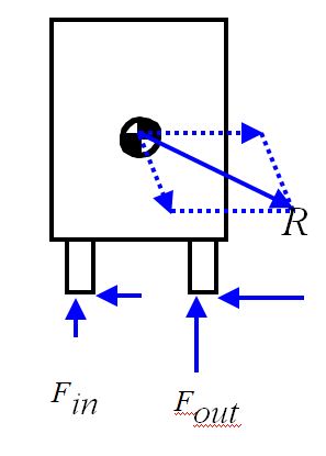
This work develops a unique Kalman
Filter
and a sensing suite that permits real time measurement of the proximity
of a vehicle to
motion-induced rollover. Instead of predicting rollover itself, we
predict the liftoff of wheels which precedes rollover. This is easier
to do while also being a more conservative approach. The basic issue is
the direction of the net non-contact force relative to the support
polygon formed by the wheels in contact with the terrain.
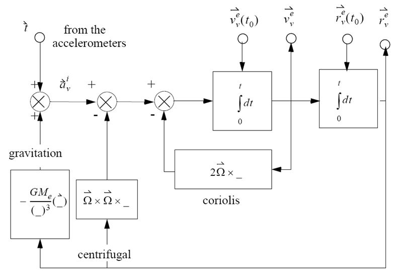
Accelerometers in an inertial measurement unit (IMU) measure this
vector quantity almost directly - but not quite. The issue is that we
need to know the inertial force direction acting at the center of
gravity (c.g.) and you can't often put an IMU right at the c.g. That
means we have to transform the acceleration to the c.g. frame.
Doing that requires 3 gyroscopes (for the centrifugal and
Coriolis terms) and maybe a real-time mass properties engine if the
vehicle articulates or moves anything - because that would change the
c.g. location. Any articulations will need to be measured and the
Coriolis term requires a measurement of velocity. Thankfully, that is
as complicated as it gets in general. Put all that into a Kalman filter
and you have a vehicle smart enough to stop itself from rolling over on
arbitrary terrain (including arbitrary slopes). Long term, any mobile
robot doing real work outdoors will probably need something like this
in it.
Potential applications include a safety system in
any robot or any man driven vehicle that is at risk of rolling over. In
the former (robot) case, an emergency stop can be issued if things get
too close to wheel liftoff. It would also make sense to predict the
stability margin using the same mathematics and predicted accelerations
rather than measured ones - in order to be preemptive. In the
latter (human) case, speed governing can be
applied to reduce the risk level but we elected to leave the human in
charge of steering in our tests.
Diaz-Calderon, A., and Kelly, A., “On-line Stability Margin and
Attitude Estimation for Dynamic Articulating Mobile Robots”, The
International Journal of Robotics Research, Vol. 24, No. 10, 845-866
(2005) [pdf]
3.0 Human Interfaces
While
fully autonomous behavior may seem like the gold standard for a robot,
they are of little use unless we can communicate with them effectively.
Long term doing a good job here will require innovations in speech
recognition, agent modeling, and situation awareness among many other
things. The work described below is focused on teleoperation - telling
a robot exactly what to do as if it were a car - but doing so from
perhaps thousands of kilometers away. 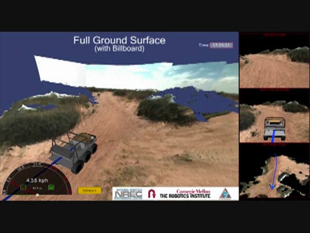
3.1 Synthetic Remote Control
This recent work in robot teleoperation is a radical new approach that
converts the environment around a robot instantly into a computer
graphics database. That is hard to do but, once done, it makes other hard problems
easy. We are able to improve remote operator situation awareness and even
remove latency with this technique. The concept relies on a new sensing
concept called colorized range sensing which is described below in
Sensing.
Click the image
to see what the operator sees while driving this robot from a kilometer away over a radio data link.
The difference between
teleoperation and
remote control is that you look
through the robot's (video) eyes in the first, and you look
at the
robot in the second. The second is much easier to do. Our approach
converts teleoperation into synthetic remote control. The operator can
drive the robot as if he were flying behind (over, around) it in
a synthetic helicopter. We can look at the robot in the context of its
surrounding terrain from any perspective. A synthetic overhead view is
nice for driving backwards into a parking spot.
There is a patent pending on this work.
A. Kelly et al., “Real-Time Photorealistic Virtualized
Reality Interface for Remote Mobile Robot Control”, to appear, The International Journal of Robotics
Research.
[pdf]
4.0 State Estimation
There are basically two methods of
position estimation: dead
reckoning and triangulation. Triangulation methods are those which
associate measurements gathered on the vehicle with some prestored map
of the area to produce a "fix" on the position of the vehicle. The map
may encode predictions of any form of radiation at any position - like
what you will see, hear, recieve on a radio antenna etc. Systems
based only on dead reckoning get more and more lost over time, so
some form of triangulation is almost always necessary in practice - if
accurate absolute positioning is desired.
4.1 Personal Navigation
This work has developed a micro inertial navigation system for people -
like a GPS for pedestrians - except it does not use GPS. The
system is quite literally an implementation of the same inertial
navigation algorithms used in a missle or a submarine, but it is adapted and made
small enough for humans to wear. The key to high performance personal navigation is zero velocity updates (zupts).
These are fake "pseudomeasurements" of zero velocity that are fed to
the system when the foot is in contact with the ground. Doing so makes
it possible to observe the biases on the accelerometers and two of the
three gyros. The vertical gyro bias remains unobservable by this
technique and that is the dominant residual source of error in many
cases. We use various radars to observe vertical gyro bias and the
system performance is much improved as a result.
Click the image to see a brief promotional video describing how it all works.
This paper provides a brief overview but I can't put it on the web site....
Al Kelly, Tamal Mukherjee, Gary Fedder, Dan Stancil, Amit Lal, Michael
Berarducci, “Velocity Sensor Assisted Micro Inertial Measurement
for GPS Denied Personal Navigation”, 2009 Joint Navigation
Conference, Orlando Florida. [pdf]
4.2 Vision-Aided Inertial Navigation
Inertial navigation is the process of
dead reckoning from indications of linear acceleration and angular
velocity. The great thing is it works anywhere in the universe where
the gravitational field is known, and it requires no infrastructure like
landmarks, beacons, satellites and their associated maps. The
not-so-great thing is it does not work well enough in most cases unless
you have extra sensors called aiding sensors. In robotics, visual
odometry is uniquely available as an aiding sensor - and it makes a big
difference.
Visual odometry amounts to a differential pose observation which is
essentially the same as linear and angular velocity readings once you
scale by time. Velocity aiding turns the short-term cubic error growth
of position variance to a linear growth . This work describes a means
to fuse the data from visual odometry and inertial navigation.
J. P. Tardiff, M. George, M. Laverne, A. Kelly, A. Stentz, “A New
Approach to Vision-Aided Inertial Navigation”, IROS 2010. [pdf]
4.3 Navigation from Floor Mosaics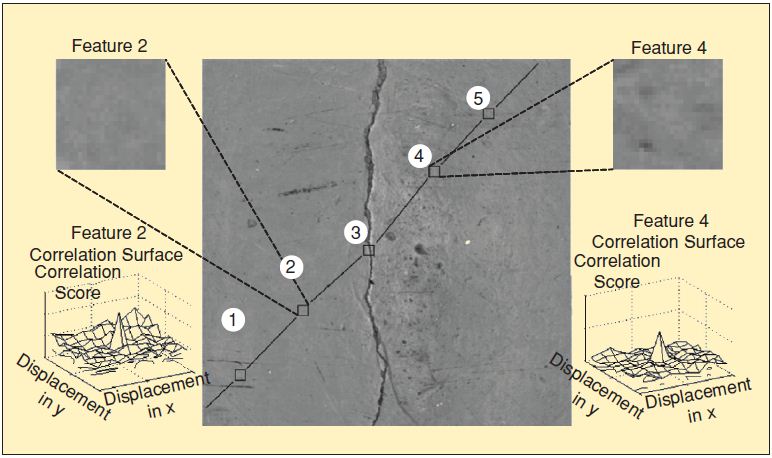
This work describes a means to
localize a mobile robot based only on
the use of imagery of the floor of the building (perhaps a factory or warehouse) in which it travels. A
camera is mounted underneath the vehicle. The first time the vehicle
drives in the building, all the images are remembered and formed into a
globally consistent mosaic. That is a problem in itself whose solution
is described in the section on
building maps with cycles.
Once the mosaic is constructed, the vehicle can then drive anywhere on
the mosaic. The guidance system matches the floor imagery in view to
the floor imagery that is predicted to be in view. It searches a
limited area around its predicted location for a match. Once a
match is found, it is used to resolve the small errors that accumulate
in the fraction of a second that passes between image acquisitions. In
this way, the system maintains a continuous visual lock on the mosaic.
Click the image
to see the system running a test. Notice the red laser light under the white vehicle near the end.
The system is a visual equivalent of the Global Positioning System
(GPS) because it uses signal correlation in order to achieve the
highest possible signal-to-noise ratio. It works even on very dirty
floors provided there is enough persistent visual texture on the floor. The
texture can be intrinsic to the floor design, like aggregate in
concrete, or it may be scratches and imperfections that persist over
time. The system was tested successfully for a week on a robot in an
auto plant with kilometers of internal roadways. A custom engineered camera and lighting system is used but
the basic concept will work without it. Repeatability on the order of
one half pixel - 2.5 millimeters in our case - is achievable. With
odometry aiding, the system can work at highway speeds. These days, you
can store enough imagery to mosaic a path across the USA on a single
DVD, so storage space for the mosaic is not an issue in practice.
This work is patented. Google "infrastructure independent position determining system".
Kelly, A, “Mobile Robot Localization from Large Scale Appearance
Mosaics”, The International Journal of Robotics Research, 19
(11), 2000.
[pdf]
5.0 Systems Theory
Building robots well is a systems
engineering exercise. For example, the capacity to competently avoid
obstacles at speed depends on the maximum range that the robot can
competently see, how fast it can react, how good the brakes (or
steering) are, and how fast it is going. Optimizing only one of these
attributes is not the most effective approach; its better to work the
whole problem from all angles.
This work studies the
interrelationships of subsystem and system level requirements (constraints),
the crafting of performance models (objectives), and highly principled and
well-argued approaches to the construction of the best achievable solution. The goal is to understand what works well and
why so that the governing relationships can be manipulated in order to
do even better.
5.1 Path Sampling
It turns out that motion planning
search
spaces can be designed in order to maximize the probability of finding
a solution in
finite time, in arbitrary environments. This result establishes a
relationship between that probability and the mutual separation of the
paths that are searched. The intuition is that two paths that are
always near each other are far more likely to both intersect the same
obstacle so if a certain path does intersect an obstacle, it is
better to search other paths next which are far away from it. In the
most general case, any fixed set of candidate paths will be a better
choice on average if they are maximally separated from each other.
Green, C., Kelly, A., “Toward Optimal Sampling in the Space of
Paths”. 13th International Symposium of Robotics Research, ISRR
07, November, 2007, Hiroshima, Japan, [pdf]
5.2 Odometry Error Propagation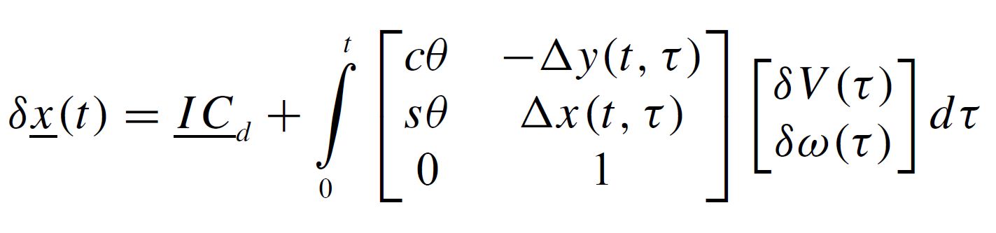
It turns out that basic odometric
dead reckoning produces a transition matrix for the linearized error
dynamics that can be written in closed form.
In some sense, that means we know everything about the linearized error
dynamics of odometry. Its an explicit integral. The integral shown
applies to integrated heading odometry - the use of measurements of
linear and angular velocity. This work establishes the fundamental
error dynamics of velocity based
dead reckoning - known in robotics as "odometry". The result
applies to both systematic and stochastic error dynamics and it applies
to
the general case of any trajectory.
The basic integrals, like the one shown, can be manipulated into
moments of arc - basic geometric properties of the path itself. These
moments are the fundamental mapping from sensor error onto errors in
the computed solution for position and orientation - and they tell us
many very interesting things:
- As a first order solution, the total pose error can be written as
the superposition of the contributions of all error sources.
- In many cases crosstrack error grows quadratically in
distance or time whereas alongtrack and heading errors grow
linearly.
- Pose error due to velocity scale error cancels out on closed paths.
- Pose error due to constant gyro bias cancels out at the dwell centroid of the path.
- Pose error due to gyro random noise is not necessarily monotone
in time - you can actually get less lost by doing the right things.
More on this in the following paper....
Kelly, A, "Linearized Error Propagation in Vehicle Odometry", The International Journal
of Robotics Research. 2004; 23: 179-218. [pdf]
5.3 Triangulation Error Propagation
This
work investigates the so-called
"geometric dilution of precision" in triangulation (and trilateration)
applications. This quantity governs the mapping from sensor errors to
computed pose errors so it is basic to understanding triangulation
systems. This work is the triangulation equivalent of the above work on
odometry. The results are very distinct from odometry. Here, the
governing equations are kinematic and transcendental so we don't have
to deal with messy integrals. The most basic insight here is that the
first order error mapping is a Jacobian matrix and any matrix produces a
linear transformation of its inputs. The basic magnifying capacity of
any matrix is related to its eigenvalues (length) and determinant (volume) and the determinant is arguably
equal to or at least the limit of the "geometric dilution of precision" or
GDOP (pronounced gee-dop).
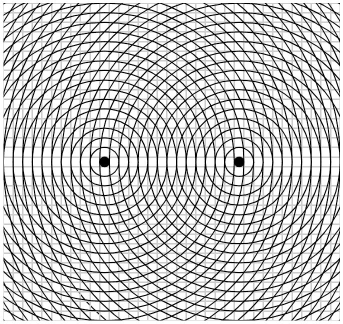
In simple cases, this is obvious graphically. The figure opposite is
the 2D analog of GPS. The dots are the satellites and the circles are
contours of constant range. The robot can be anywhere in the plane. Notice how the circles are larger on the
line between the satellites and larger near the edges of the figure.
All that falls naturally out of the mathematics.
Among the insights that this work produces:
- GDOP is infinite on the line between landmarks in most cases. That's why operating between landmarks is so poorly conditioned.
- Range observations are fundamentally better than angular ones from the point of view of precision.
- Hyperbolic navigation is one of the most stable forms of
triangulation - in the sense that GDOP varies smoothly and minimally
and there are no singularities. Marine radio navigation used to be
based on this principle but most systems are turned off today.
Kelly, A., “Precision Dilution in Mobile Robot Position
Estimation”, In Proceedings of Intelligent Autonomous
Systems, Amsterdam, 2003. [pdf]
5.4 Perceptive Obstacle Avoidance and Mapping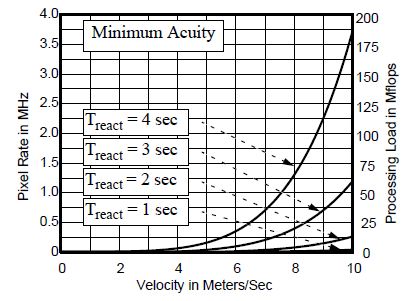
This work looks at what precisely is
needed, in terms of performance, for a mobile robot to be capable of
avoiding obstacles at speed. One of many analyses considers the
computation
necessary, and how that computation
requirement varies with speed. In rough terms, you have to put a few
pixels on the
obstacle to see it. The faster you drive, the farther away you have to
see it. The farther away the obstacle, the smaller the pixels need to
be - but the
sensor field of view is typically fixed. Express all that in algebra
and
you get the graph opposite. Depending on your assumptions, the
computation necessary to avoid obstacles grows with the eight power of
vehicle velocity. If you are more clever about it, you can reduce the
speed dependence to a merely quadratic term in velocity. In other
words, doubling the speed can require 256 times as much computation or
4 times as much - depending on how you design the perception
system.
Kelly, A., Stentz, A., "Rough Terrain Autonomous Mobility – Part
1: A Theoretical Analysis of Requirements", Autonomous Robots, 5,
129-161, 1998. [pdf]
5.5 Efficiently Building Maps with Cycles
This work considers the problem of building maps from large datasets which
contain relatively few cycles. In that case, some very efficient
methods
exist. There are many ways to formulate map building. This one uses
nonlinear programming - also known as constrained optimization. The
objective function to be optimized is the mismatch error at image
overlaps and the constraints are the expressions that the composite
transform around a closed loop must take you precisely back to where
you started. In other words, the composite transform is the identity transform. When there are few constraints,
it is computationally efficient to
not substitute the constraints into the objective. The solution in that case is the one you use when you
can't
substitute the constraints into the objective - Lagrange multipliers.
By keeping the constraints explicit, the matrix to be inverted remains
diagonal and enforcing loop closure in very large maps of hundreds of
thousands of images can be done in a fraction of a second. Extensions
to incremental / recursive / on-line algorithms are possible.
Kelly, A. Unnikrishnan, R., “Efficient Construction of Optimal
and Consistent Ladar Maps using Pose Network Topology and Nonlinear
Programming, In Proceedings of 11th International Symposium of
Robotics Research (ISRR'2003), Sienna, Italy, November 2003.
[pdf]
6.0 Off-Road Mobility
Off road
navigation deals with the challenge of making robots which can drive
themselves competently outdoors. This problem is significantly more
difficult than indoor movile robot navigation in many ways. An
inadequate vehicle design will mean that even moving will be a
challenge on wet soil or on slopes. Holes and cliffs may exist that
cannot be seen, without tremendous effort, until its too late to avoid
them. Tall grass may hide lethal objects that will ruin or entrap the
tires or throw the tracks. Many natural environments are complicated
mazes that are hard to solve without a map. Despite the navigation
revolution of GPS, it does not work under dense tree canopy, so its
also easy to get lost. Outdoor mobile robots have a lot to cope with.
6.1 PerceptOR / UPI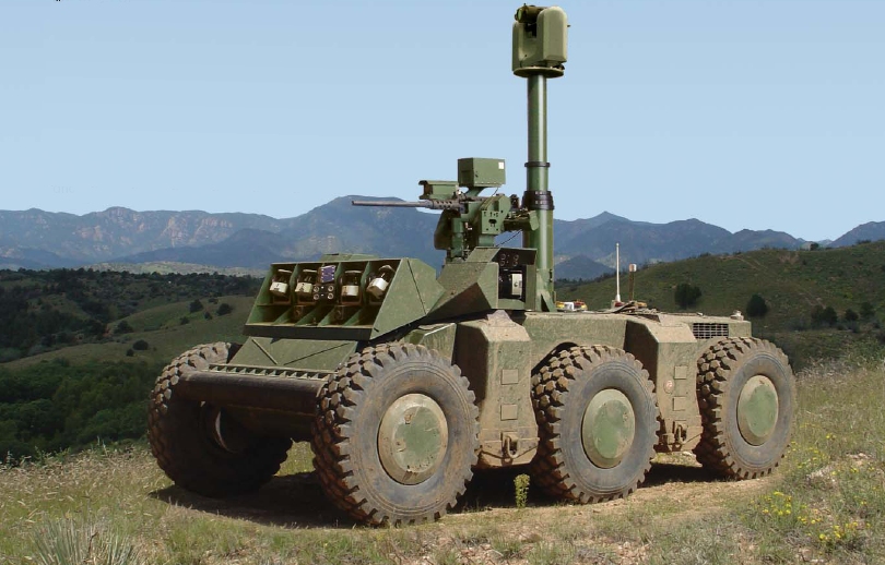
The PerceptOR robot was capable of
impressive levels of autonomy in off-road environments. This system was
tested for weeks at a time on army bases throughout the USA. The final
versions of this system were used on the Crusher vehicle shown opposite
and a typical day of testing included 50 kilometers of autonomous
motion with human interventions required much less than once per kilometer.
Click the image
to see Crusher featured on Youtube.
Many researchers worked on this system and they, and their work, can be
found on the RI projects pages. Look for the UPI project.
Kelly, A., et
al., “Toward Reliable Off-Road Autonomous Vehicles Operating in
Challenging Environments”, The International Journal of Robotics
Research, Vol. 25, No. 5–6, pp. 449-483, June 2006.
[pdf]
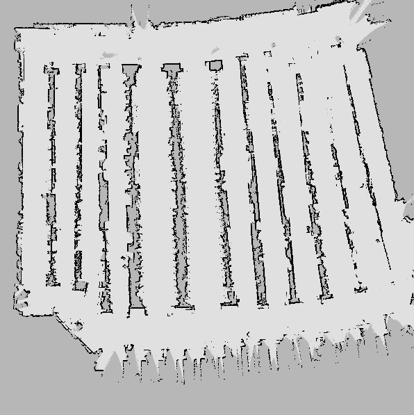
6.2 Demo II Ranger System
An early effort in UGV navigation
that produced continuous obstacle avoidance at 15 kph in 1990.
The Ranger system is an optimal control approach to obstacle avoidance.
The objective to be minimized is deviation from a preferred trajectory
which may be specified as a direction, a path, a curvature like straight ahead, etc.
Obstacles in this system are not discrete spots or regions on the
ground. Rather, they are regions in state space - which includes
velocity, curvature etc. This approach makes it easy to incorporate
things like rollover hazards into the computation. Hazards are
typically treated as constraints - they do or do not eliminate certain controls from
consideration. Any controls that were not eliminated are scored for
utility (objective function) and the best is selected. This process is repeated at 10 Hz or so.

At high speeds, the complicated response of the vehicle to its inputs
cannot be ignored. This system uses explicit forward simulation in
order to ensure that vehicle dynamic models are satisfied. In other
words, the system knows how long it takes to turn the steering wheel
and it takes that into account. This approach means the search for the
right input is conducted in input space. That makes it hard to sample
effectively but sampling is not so important at this level of motion
planing. The
Urban Challenge lane following controller does sample
effectively and it respects environmental constraints like lanes. It
came later but that technique also requires more computation.
Ranger also used many schemes to limit the computation required of
perception. Notice the adaptive regions of interest in the figure
opposite - these adapt automatically to the terrain geometry and vehicle speed. The
result of that adaptation is more competent operation at higher
speeds. A key idea here is
computational stabilization of the
sensor. That is a kind of
active vision approach that finds the
data of interest in the image with minimal computation. As computers
get faster we tend to add more pixels to sensors so this technique remains
relevant today.
Kelly, A., Stentz, A., "Rough Terrain Autonomous Mobility – Part 2: An Active Vision,
Predictive Control Approach", Autonomous Robots, 5, 163-198, 1998. [pdf]
7.0 Calibration and Identification
These two terms mean the process of discovering the values of unknown
parameters which are used in system models. This work concentrates on
the problem as it occurs in mobile robot mobility and estimation
systems - that is - the calibration of differential equations that
describe motion, or the measurement of motion.
Long term, mobile robots need to be able to calibrate themselves
automatically - just like an infant learns how to use its own arms
and legs by experimentation.
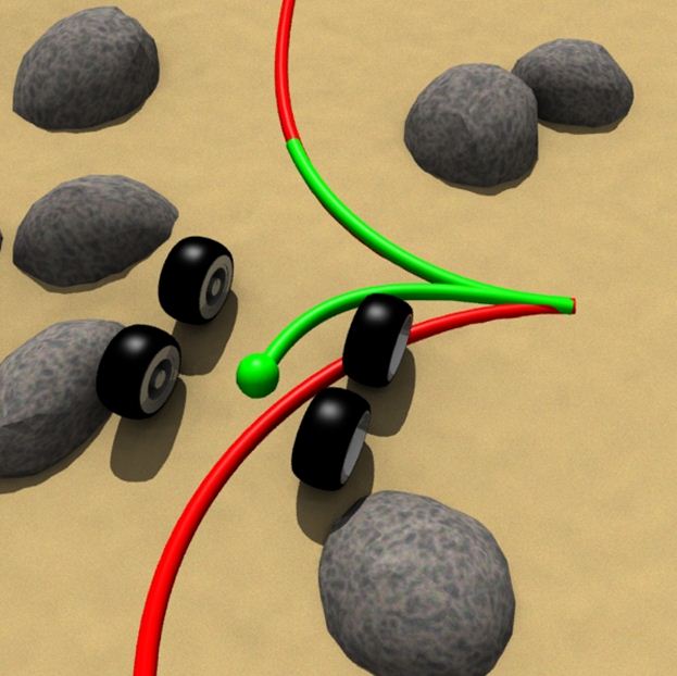
7.1 Identifying Dynamic Models
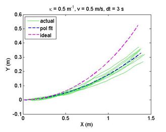
This work develops a means to calibrate the mapping between inputs
(controls) and outputs (state) for a vehicle. The formulation is to
model only the deviations (perturbations) from a nominal model and to
assume driving disturbance inputs cause those deviations.
Both systematic and stochastic disturbances can be calibrated.
Observations are formed from the differences between the system
trajectory predicted based on the present model and the trajectory
which was observed to occur. That is, at regular intervals, the system
observes where it is now and it considers where it would have predicted
itself to be now if it had predicted it a few seconds ago. These
predictions involve integrating the perturbative dynamics.
The disturbances are parameterized functions of the inputs and this
means that the entire mobility envelope of the vehicle is being
calibrated. The models are calibrated in real-time while the vehicle
drives so whatever trajectories the system is executing are used. The
figure shows the short term response of a skid steered vehicle to left
turn commands. Clearly the vehicle is slipping sideways because the
green lines are all to the right of the red - and the red was asked for.
The essnetial process is to write the slip velocities in terms of
unknown parameters and solve for the parameters. We do that with a Kalman filter.
F. Rogers-Markovitz, A. Kelly, “Real-Time Vehicle Dynamic Model
Identification using Integrated Pertubative Dynamics”,
International Symposium on Experimental Robotics, June 2010. [pdf]
7.2 Identifying Dead Reckoning Systems
This work is motivated by a very
pragmatic need to calibrate dead reckoning systems for mobile robots.
The result can calibrate both systematic and stochastic models - so it
can produce not only calibrated estimates of robot motion but also of
the uncertainty in those estimates. The basic mathematical techniques
include linearizing the system dynamics and then using the
linearized error dynamics, and the linear variance equation. The
technique also uses arbitrary motions to a single known point from an
arbitrary origin in order to minimize the need for (expensive and
difficult to acquire) ground truth information. For stochastic
modeling, the total probability theorem is used in order to avoid the
need to repeat the same trajectory over and over. Arbitrary
trajectories can be used instead. In fact, the results are better if
the trajectories are as different as possible.
Kelly, A., “Fast and Easy Systematic and Stochastic Odometry
Calibration”. In Proceeedings of the International Conference on
Intelligent Robots and Systems (IROS), Sendai Japan, September 2004. [pdf]
8.0 Automated Guided Vehicles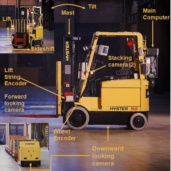
AGVs are (typically) indoor robots
that move material from place to place. These may be configured as
tugs, unit loads, or forked AGVs. The market for these mobile robots is
well established.
8.1 Infrastructure-Free AGVs
An effort to make an AGV which can
guide itself entirely based on vision and no plant infrastructure.
There were four visual servos. One was used to guide the gross vehicel
motion. Another was used to pick up objects and parts racks with the
forks. A third was used to stack racks on top of each other. A fourth
was used for navigation inside (while loading and unloading) shipping
containers.
Kelly, A.,Nagy, B. ,Stager, D.,
Unnikrishnan, R., “An Infrastructure-Free Automated Guided
Vehicle Based on Computer Vision”, IEEE Robotics and Automation
Magazine. September 2007.
[pdf]
9.0 Sensing
Some say that better sensors are all we need for better robots.
Others say they will never be good enough. A few research programs have
investigated the construction and performance of new sensors.
9.1 Inertial Navigation Systems
We
have developed our own custom low-cost strapdown inertial navigation
system for mobile robots. The system is based on a high performance
(tactical grade) micro electromechanical system (MEMS) inertial
measurement unit (IMU). Mobile robots place unique demands on the
performance of pose estimation systems due to the unique demands
of perception and mapping tasks. A robot needs to know precisely which
way is up in order to correctly assess the slope of the terrain
in view. Waypoint following typically depends on an accurate global
position - particularly if the robot is blind (has no perception
system). Mapping requires a smooth pose estimate and mapping is
particularly sensitive to attitude errors. If scanning sensors like
scanning lidars are used, it becomes critical to be able to associate
an accurate position and orientation of the lidar sensor with every
lidar pixel. This system is designed to address all of these unique demands.
Mobile robots also provide unique opportunities to aid a guidance
system. Odometry is almost always available and most perception sensors
can be harnessed to help out. The system can accept these unique
robotic aids as well.
This system is now being sold commercially - which is why this section
is a little less technically detailed than the others. I am not allowed to put its picture here.
9.2 Colorized Range Sensors
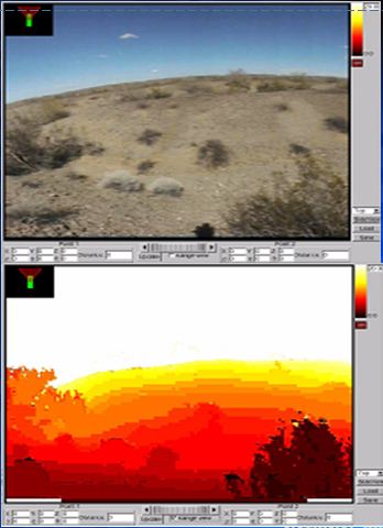
The NREC colorized range sensor is a good contender
for the right sensor modality for mobile robot perception. Such sensors
produce a red-green-blue-depth image so that both the appearance and
the geometry of the scene is known for every pixel. The data is
registered at the pixel level. The original motivation for this sensor
modality was obstacle detection - rocks and bushes can have
similar appearance but the bush will be penetrated by the lidar
beams and the rock will not.
Later, we have found more uses for these sensors. In particular they
are also perfect for
virtualized reality - the process of turning a
real scene into a computer graphics model. This is done essentially
instantly, and essentially in hardware, using colorized range sensors.
A. Kelly, D. Anderson, H. Herman, “Photogeometric Sensing for
Mobile Robot Control and Visualization Tasks”, 23rd Convention of
the Society for the Study of Artificial Intelligence and Simulation of
Behavior, AISB 2009, Edinburgh, Scotland. [pdf]
9.3 Flash Ladar Sensors
This paper characterizes the performance of two flash lidar sensors. This an important up-and-coming sensor modality for robots.
Anderson, D., Herman H., Kelly, A., “Experimental
Characterization of Commercial Flash Ladar Devices”, In
Proceeedings of International Conference on Sensing Technologies,
November 21-23, 2005 Palmerston North, New Zealand. [pdf]
9.4 Scanning Lidar Sensors
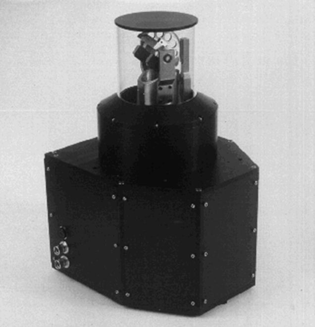 This effort, conducted in conjunction with Quantapoint (http://www.quantapoint.com)
produced a scanning laser radar sensor of very high accuracy (mm range
accuracy). It has an omnidirectional horizontal field of view with no
blind spots. The novel scanning mechanism is patented.
Quantapoint has been in the as-built modelling business for many years.
This effort, conducted in conjunction with Quantapoint (http://www.quantapoint.com)
produced a scanning laser radar sensor of very high accuracy (mm range
accuracy). It has an omnidirectional horizontal field of view with no
blind spots. The novel scanning mechanism is patented.
Quantapoint has been in the as-built modelling business for many years.
 Back to Robotics Institute Homepage