
Quick Summary
You will need to download and install a set of 3rd party software to analyze and visualize the data.
Capturing the images: Use digital camera to take images in sequence, in a pattern that sees the scene from all possible angles.
Process the images for reconstruction: Install VisualSFM and CMPMVS. Take advantage of these applications to get 3D models from images, as shown in the figure below (left to right process).
Measurement and analysis: Use VisualSFM, Meshlab and CloudCompare tools to visualize and measure the deformation, as shown in the figure below (the bottom half).
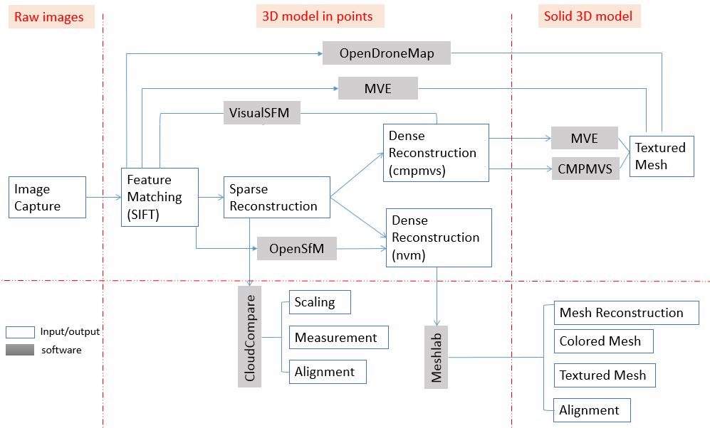
Image Capturing
Recommended equipment:
Digital camera is recommended. We used Samsung Galaxy camera, which captures images that are 4608 pixels wide and 3456 pixels high; and videos that are 1920x1080. The idea is to get better quality images. Higher resolution images usually help preserve detail and get better reconstruction result.
The images do not have to be taken with a single camera (i.e. differences on resolutions, or image sizes, are acceptable). Note that distortion of the lens may affect the result; modified photos may also cause inaccurate result.
Image taking approaches:
The algorithm needs to,
Ø recognize the scene,
Ø view the scene from many angles to understand the three dimensional relationship.
Thus, the general idea is to take images from slowly translating angles.
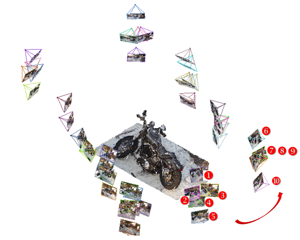
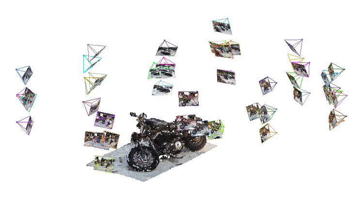
Below is an example of taking pictures of a motorcycle. In the center is the motorcycle dense reconstruction result in VisualSFM. The surrounding pyramids shows the 3D position of the images taken.
 |
 |
Basic rules:
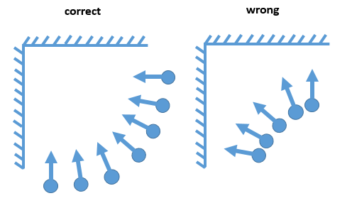
- Start at one spot, take three images at high, middle, low position. Move to the next spot, take three images. Walk roughly in a circle surround the scene/object. Imagine the scene/object as the center of the circle; the camera's viewpoint casts a ray to the scene, like the radius of the circle. Try to keep two rays within 30 degree angle. Repeat until disclosure the circle.
- For a feature to be successfully reconstructed, it has to be seen by least three cameras. The more, the better.
- All cameras are pointing to the scene/object (the Harley in this case).
- All cameras have a similar distance from the scene/object. The scene/object should not look too large or too small. Ideally, frame your scene/object in the middle 1/3 to 2/3 of the picture.
If you want particular detailed features, take multiple pictures at equal intervals while slowly approaching the feature of interest. Do not move your camera dramatically in one single direction. This is to make sure the program could understand and relate the detailed feature to the whole scene.
We recommend taking a new set of images for a separate reconstruction of the detailed feature, unless it has to be part of the general large-scale scene/object. - Reflections and shadows do affect the program’s judgement. Try to take more images from different viewpoint to secure the reconstruction.
- More features would help locate the camera. Always include surrounding features. For example, a piece of white wall is featureless; a door frame would be feature on the white wall. A car hood itself is featureless (too smooth and uniformed); a zoom-out picture including side mirrors, windshield, ground, tires, etc. would make it easier for the program to ‘understand’ and to locate the hood.
Alternatively, one can take videos of the scene/object, or shoot in burst mode (continuous high speed shooting).
One way of video frame extraction is to use free open source software GIMP&GAP. Please refer to this video for detailed instructions. Download and install GIMP, GAP, and GIMP extensions, following the link provided in the video.
We recommend moving the camera in similar manners – walking around in a circle while moving the camera up and down.

Software Installation
Software and hardware requirement:
The instructions are designed for Windows (64-bit) operating system with NVIDIA CUDA-enabled GPU. Contact us if your platform is different.
An alternative for VisualSFM+CMPMVS is Multi-View Environment (MVE). It works on Linux OS and is distributed under less strict license. For more details on MVE usage and performance, click here.
Download and install a set of 3rd party software to analyze and visualize the data:
- VisualSFM
- CMP-MVS (requires CUDA)
- Meshlab
- CloudCompare
Install VisualSFM:
- Check the system properties.
On your computer, go to “Computer”> “system properties”.
Check and make sure your machine has a 64-bit operating system. - Get VisualSFM windows binaries from here:
http://ccwu.me/vsfm/
Go to the Download section and download the first one “Windows*”. Click on ’64-bit’, which matches your operating system.
Download from the second option “Windows”, if you do not have CUDA.
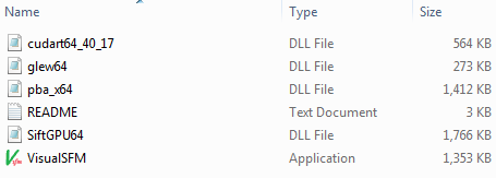
Download the version that matches with your operating system. Save it to a folder of your choice. Unzip the package. It should look like below, where the VisualSFM application locates:
- Get the CMVS/PMVS binaries from here:
http://code.google.com/p/osm-bundler/downloads/detail?name=osm-bundler-pmvs2-cmvs-full-32-64.zip
Unzip the package. And then put cmvs.exe, pmvs.exe, genOption.exe and pthreadVc2.dll in the same folder as the VisualSFM application, which you got in step 2.
You will find these files in the directories:
.../osm-bundler/osm-bundlerWin64/software/cmvs/bin and
.../osm-bundler/osm-bundlerWin64/software/pmvs/bin
Install CMPMVS:
CMPMVS can be found here:
http://ptak.felk.cvut.cz/sfmservice/websfm.pl?menu=cmpmvs
As CMPMVS requires a NVIDIA CUDA-enabled GPU, it may not work on some computers. An alternative way to generate a mesh reconstruction is using Meshlab. See the Meshlab section for details.
Download the latest version:
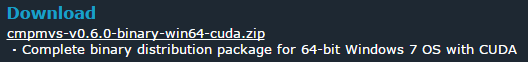
Read the readme.txt carefully. Make sure you have installed:
-
Visual Studio 2008 x64 redistributable: http://www.microsoft.com/en-us/download/details.aspx?id=15336
-
Latest GPU driver: http://www.nvidia.com/Download/index.aspx?lang=en-us
Install Meshlab:
Meshlab can be found here: http://meshlab.sourceforge.net/
When the Meshlab setup wizard started, click on 'Next', 'I Agree', and accept the default path, and 'install'.
You might have errors (e.g. “missing Microsoft Visual C++ 2008 SP1 Redistributable Package (x64)”). It may because some packages are not installed on your computer. Download the missing package and install. The problem should be fixed.
Install CloudCompare:
CloudCompare can be found here: http://www.danielgm.net/cc/
On CloudCompare Download page, click to download the CloudCompare 2.6.1 installer version for Windows 64 bits (or Windows 32 bits based on your operating system).
When the downloading completes, double-click on the installer. Click 'Run' and 'Yes', if your system pops up windows for security reasons.
When the CloudCompare setup wizard window shows. Keep clicking 'Next' (for four times). Then Click 'Install'.
Dense Reconstruction
The dense reconstruction is done using VisualSFM.
Double click on the VisualSFM application icon ![]() to open VisualSFM. You can find the application in the unzipped VisualSFM folder. See ‘Install VisualSFM’ section above for details.
to open VisualSFM. You can find the application in the unzipped VisualSFM folder. See ‘Install VisualSFM’ section above for details.
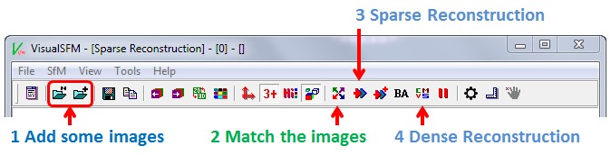
Follow the first four steps below.
Cite: http://ccwu.me/vsfm/
- Click
 to load your images.
Image name should contain only numbers and letters. Special characters may cause VisualSFM reconstruction failure.
Browse to your image folder. Press ‘ctrl’ + ‘A’ on your keyboard at the same time to select all images. Click OK.
The loading may take a few seconds, depending on the number of images. - Click on the button. The process may take seconds to minutes, depending on the number of images.
- Click on the button. After the process terminated, you can drag the model by pressing the left mouse button, and rotate the model by pressing the right mouse button and dragging. Also, you can read the information in the log window (on the right). It tells you how many models are reconstructed. Ideally, we want one complete model. The fewer models it generated, the better.
- Click on the button. If you got multiple models in previous sparse reconstruction process, press ‘Shift’ and click. This creates dense reconstruction for all models.
In the popped up window, name your dense model. Leave the ‘Save as type’ in its default. Click ‘Save’. The dense reconstruction process may take 30 minutes to complete. The result can be visualized in VisualSFM, Meshlab, or CloudCompare. See the measurement section for details.
Mesh Reconstruction
The CMPMVS takes the dense model generated by VisualSFM, and do mesh reconstruction. See the advanced features (look for 'How to do mesh reconstruction in Meshlab') on how to generate mesh with Meshlab.
- Repeat to the first three steps in Dense reconstruction.
- Click on the
 button. In the popped up window, look for ‘Save as type:’, then select the second option, i.e. ‘NVM -> CMP-MVS’. Name your file and click ‘Save’. This process may take a few seconds.
 - Browse to the newly exported .nvm.cmp folder and open the mvs.ini file with a text editor (like notepad). In the [global] section, ensure that the directory in the line dirName=”<path_to_your_folder>.nvm.cmp\00\data\” is correct for the machine you will be running CMPMVS on, including the trailing slash (“\”). If you change machines, you will need to change this to the absolute path of the 00\data\ folder.
- Run CMPMVS from the command line as shown below.
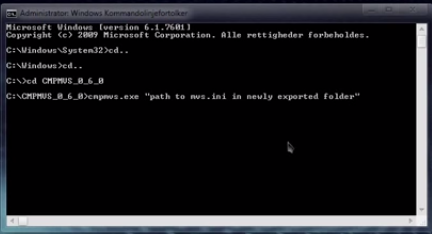
In command line, change directory (type ‘cd’ followed by a space) to the folder where CMPMVS executable is installed/located. To run the application, type CMPMVS.exe, followed by a space, followed by the directory of the mvs.ini file. To find the directory of the mvs.ini file, browse to the .nvm.cmp folder (which is newly exported from VisualSFM steps) > 00, copy the route and paste into the command line, and type the name of the mvs.ini file. Hit Enter to run with default settings.
The command line example:
C:\user\...\cmpmvs\CMPMVS_6>CMPMVS.exe E:\...\00\mvs.ini
Note that there should be no space in the path to mvs.ini file. Otherwise error occurs.
You can also add more options to change parameters.
For example, put another single space, and paste the options you want. The options can be found in readme file under CMPMVS root folder. Hit Enter to run CMPMVS with your settings.
The command line example:
C:\user\...\cmpmvs\CMPMVS_6>CMPMVS.exe E:\...\00\mvs.ini DoGenerateVideo=True.
CMPMVS process may run for several hours. When it’s finished, the command line status should be like:
C:\user\...\cmpmvs\CMPMVS_6>_
The reconstruction results are saved in the ~\00\data\_OUT\simplified10 folder. The colored mesh is named ‘meshAvImgCol.ply’. The Textured mesh is named ‘meshAvImgTex.wrl’. In case you want a denser reconstruction, go to the ~\00\data\_OUT folder to find the original files with same names.
Open them in Meshlab or CloudCompare. See the measurement section for details.


CMPMVS TroubleShooting:
-
Crashes at
“Processing input images
Loading input data”
Possible solution: The dirName in the [global] section of mvs.ini does not have an absolute path to the 00\data\ folder. Ensure that the path is correct, absolute (starts with C:\), and ends with a trailing slash (\).
-
Crashes immediately with “The application was unable to start correctly (0xc000007b). Click OK to close the application.”
Possible solution: Copy C:\Windows\System32\D3DX9_43.dll to the same folder as CMPMVS.exe and rename it to d3dx9_42.dll
See https://groups.google.com/forum/?fromgroups#!topic/cmpmvs/J33ZitOyj78.
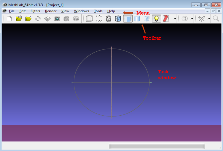
Visualization in VisualSFM
When VisualSFM is open, two windows present. The one on the right is a ‘log window’; the left one is referred to as ‘task window’.
Tool bar:
 Menu:
Menu:

Operate with mouse, keyboard, and menu buttons
Drag (press and do not release) the left mouse button to move the model.
Drag (press and do not release) the right mouse button to rotate the model.
Use mouse scroll wheel to zoom in/out.
Use the buttons  to switch between 3D views and image thumbnails.
In dense mode, click  the show/hide features button to see the cameras (i.e. images). Press ‘Ctrl’ and scroll the mouse wheel to zoom the cameras.
In sparse mode, press the up/down arrow key on keyboard to see different models.
View dense reconstruction result
After the dense reconstruction process complete, do not quit the program. Click anywhere inside the VisualSFM task window to make sure it’s activated. Now press ‘Tab’ on the keyboard to see the dense reconstruction. Press ‘Tab’ again to switch to sparse reconstruction.
Load a previous reconstruction
Sometimes you start the VisualSFM and would like to see a previously reconstructed model (a dense reconstruction).
Click on  the Load NView Match button. Browse to the location where you stored the (dense_file_name).nvm.cmvs folder. There should be a separate (dense_file_name).nvm file in the same directory. Click on the .nvm file (not the folder). Click ‘Open’. Wait for the loading process to complete. Then activate the task window. Use ‘Tab’ on keyboard to switch between sparse and dense reconstruction.
Open another model in new window
You can open multiple models in VisualSFM. This is useful when you want to roughly see the difference of two reconstruction models.
In VisualSFM, go to File > New Window to open a new task window. Load a different model here.
Clean up points in VisualSFM
Press F2 in dense mode. Drag with mouse to select unwanted points. Press Delete on keyboard to delete.
Visualization in Meshlab
Import mesh reconstruction
To open and view a mesh reconstruction, click on the import mesh button on the toolbar. Click 'open' to import it.
Specifically, to open and view the mesh reconstruction done by CMPMVS, click on the import mesh button . Browse to the reconstruction results saved from the CMPMVS process. In most cases, browse to the ~\00\data\_OUT\simplified10 folder. The colored mesh is named ‘meshAvImgCol.ply’. The Textured mesh is named ‘meshAvImgTex.wrl’. In case you want a denser reconstruction, go to the ~\00\data\_OUT folder to find the original files with same names. Import them.
Operate with mouse, keyboard, and menu buttons
In case you don’t see the model in the task window, press ‘ctrl’ + ‘H’ on the keyboard to reset the view.
Drag the left mouse button to rotate the model.
Press and do not release ‘ctrl’, and meanwhile drag the left mouse button to move the model. Or you can press the mouse scroll wheel, instead of scrolling, and drag to move the model.
Scroll the mouse wheel to zoom the model.
Use  on the toolbar to turn on/off the light. This does not modify the model. Make it on or off, whichever gives a better visual effect.
Use
on the toolbar to turn on/off the light. This does not modify the model. Make it on or off, whichever gives a better visual effect.
Use  to view the model in different mode. Again, this does not modify the model. They are just different ways to view the model. The last one has to be enabled to see the color/texture information. The second last renders a smoothed model. The third from the right renders the triangle faces in the model. The first one from the left shows only the bounding box. The second one from the left shows the vertex points of the model. You can also switch these mode from the Layer Dialog.
Enable the Layer Dialog
Click on  button on the toolbar, if the Layer Dialog is not visible by default.
Select to activate layer
In the Layer Dialog, click to select the layer you would like to clean up. The selected layer will be highlighted. Mostly any tasks only affect the selected layer, unless in cases of aligning, etc.

Clean up point cloud or mesh in Meshlab
Sometimes we need to remove unwanted points:
1) Surroundings that are not part of the scene/object
2) Detached points scattered around the scene/object
3) Noise
Select (highlight) the layer you want to clean up.
Use 'Select Vertexes'  to select unwanted area. The selected area are highlighted in red.(You can also use
  to select points on a plane. This is useful to remove points inside the car.)
Press Shift to subtract selections (deselect). Press Ctrl to add selections (not very easy to control with plane selection mode, helpful when using 'select vertexes').
After selecting, click on the button again to stop selection mode. This is to be able to rotate the model and check, before removing the points. Click  to remove the selected area. Repeat until this layer is cleaned up.
Note: On some computers, Meshlab stops responding when selecting starts. In this case, the selection can be done if you keep pressing the monse button while Meshlab is not responding and releases it after Meshlab responds again. i.e. the select function is too slow.
Save the layer
Make sure to save after every step. This can also prevent Meshlab crashing from memory overflow.
To save to the original layer, simply clicking  the save button.
To save as a new layer, go to file> export mesh as… Give a different name to your layer and save it.
Analysis in CloudCompare
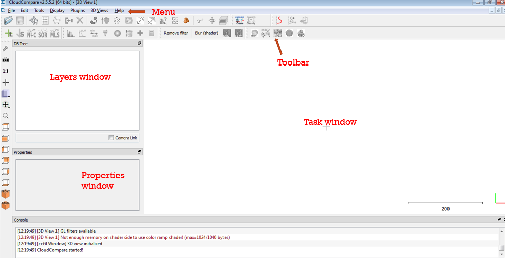
Change the bakcground color of Task window
The default task window background color is blue. You can change it by going to Menu > Display > Display settings. Click to unfold the tab 'Colors and materials'. Under Colors section, click on the blue button next to 'Background'. Change the color to white. Click 'Apply' and then 'Ok'.
Open files in CloudCompare
Open CloudCompare. From the toolbar, click  to open the file. Change the file type to ply mesh.

Browse to proper location. Click open to import.
If you have multiple files to open, press ‘ctrl’ on the keyboard, and select them. Click open to import.
Click ‘Apply’ in all the popup windows.
Combine multiple files in CloudCompare
The Merge function combines all files into one single file.
You may need to merge the mode when one model is so large that VisualSFM saved it into several option-xxxx.ply files, which can be combined into option-all.ply.
You may also need it after segmenting your model into pieces.
In the DB Tree window, press ‘ctrl’ while clicking and selecting all the option files:

In the toolbar, click  the merge button.
In the toolbar, click  the save button to save it in ~(yourfilename).nvm.cmvs /00/models folder as option-all.ply
Operate with mouse, keyboard, and menu buttons
Press and drag the left mouse button to rotate the model.
Press and drag the right mouse button to move the model.
Scroll the mouse wheel to zoom.
Select to activate layers
Unlike Meshlab, CloudCompare allows users to select and work with multiply layers. Press ‘ctrl’ and click on the layers to select. Release 'ctrl' when your selecting finished. Make sure you are selecting the Cloud, not the folder.
Turn on/off layers
Check/uncheck the box in front of the file to turn on/off the layer. This controls only the display of the file, with no modification to the file itself.
Clean up or cutting models in CloudCompare
Segmentation can be used for cleaning models, or selecting certain portions of models.
Click on  ’segment’ tool from the toolbar.
In the Task Window, left click to set the start point, click again to set another point. Click repeatedly to ‘draw’ a polygon. When you finish setting the boundary, right click to release the cursor.
In the segment menu bar, choose  to keep the inner part of the polygon and accept the changes by clicking
  . Everything inside your polygon will be saved in a new Cloud layer.
Similarly, choose  to keep everything outside of the polygon and accept the changes by clicking . Everything outside your polygon will be saved in a new Cloud layer. i.e. In the newly saved layer, everything inside the polygon has been removed.
Click  to quit the segmentation session.
You can also use the Merge tool to combine several segmented layer back together.
Rotate the model and repeat the segmentation session until getting a satisfactory model.
Save a model
Always select the layer in the Layers Window to save. Some tools may create new layers, for example, segmentation tools. Check the box before each layer to turn it on/off. Make sure you are saving the right layer.
Use the save button on the toolbar to save your work. Give your layer a new name, and it will be saved as a new file. Otherwise a window will pop up asking whether to replace the original file. It’s recommended to save files in ASCII format. You can save it as Binary to save space, if no further notepad editing required.
Align two models in CloudCompare
Say we want to align two planes: the blender plane and the table plane.
Load both plane layers. Select both the blender plane and the table layer. Align  the blender plane to the table surface. i.e. the reference is table surface cloud.
If one layer has true scale information, it’s recommended to set this layer as the reference, so that the real-world scale is preserved.
Check the box to allow ‘adjust scale’. This rescale the aligning layer to match with the reference layer.
Left click to select one anchor point. Click on the corresponding point on the other model. The program will align the models based on the anchor points. Try to be as much accurate as possible.
Drag with left mouse button to rotate the model. Scroll the mouse wheel to zoom. You can also check/uncheck the box to show/hide the layer.

When more than 4 points are selected on each model, the ‘align’ button will be enabled. Click it to see the result. Add more points for better alignment result. Click to accept the result. Save the aligned layer.
Measure distance on point cloud
In CloudCompare, load the model. Select to activate the model. Use  from the toolbar, select the mode
  to measure the distance of two points. Click on one point. Click on the second point. Click to see the distance.
Scale point cloud in CloudCompare
In CloudCompare, load the model. Select to activate the model. We use a scaling factor to scale the model. The scaling factor Sf=Dactual/Dtarget.
To find Dtarget, use from the toolbar to measure the distance (Dtarget) of two points.
The actual distance is Dactual.
Calculate the scaling factor.
Go to menu, Edit > Multiply/scale: in the fx, fy and fz fields, enter the Sf factor (same for all dimensions).
Measure distance/ accuracy of two point clouds
1) Load the two point cloud layers.
2) Press Ctrl key on the keyboard, and select both layers in the Layer Window. Now you need to cut the two layers into exact same size. Select both layers and cut them together, using the tools mentioned in ‘Clean up models in CloudCompare’ above.
3) Press Ctrl key to select the new segmented layers. On the tool bar, click the button for  ‘compare cloud/cloud distance’. In the pompt-up window, see if the parameters on each tab are proper. We normally keep the ‘General parameters’ at the default value.
4) On the third tab, click Compute to get the result.
5) You can view the histogram by clicking the  ‘Show histogram’ button in the tool bar.
6) Save your segmented layers.
Alternative: Measure distance/ accuracy of two point clouds with PCL(Point Cloud Library)
There are scripts available to 1) convert ply to pcd files, and 2) do incremental registration. The incremental registration algorithm alsohas the option to use hand picked initial points.
PCL approach automates the point cloud registration.
Edit and customize the scalar color in CloudCompare
Select the layer, in the Properties window, scroll down to the ‘Color Scale’ section. Click the setting button  on the right to the current color scale. Click ‘copy’ to copy and edit customized color scalar. Switch the mode ‘relative/absolute’ to better measure the scaling. For example, using absolute allows user to set a bar at 2 centimeter.
Under ‘Color Scale’, check the visible box to view the legend bar.
on the right to the current color scale. Click ‘copy’ to copy and edit customized color scalar. Switch the mode ‘relative/absolute’ to better measure the scaling. For example, using absolute allows user to set a bar at 2 centimeter.
Under ‘Color Scale’, check the visible box to view the legend bar.

Notes on errors
Scenario 1: CMPMVS crash Error r128 -- Absolute path issue
In the 00 folder, open the mvs.ini file with wordpad or any text editor. Note the dirName:
[global]
dirName="C:\Users….\test.nvm.cmp\00\data\"
prefix=""
imgExt="jpg"
ncams=1475
width=1280
height=720
scale=1
workDirName="_tmp"
doPrepareData=TRUE
doPrematchSifts=TRUE
doPlaneSweepingSGM=TRUE
doFuse=TRUE
nTimesSimplify=10
and check whether it is the correct directory you typed (copied) in to the cmd. Correct it to be the same as it’s current directory. Savae it.
Scenario 2: CMPMVS crash Error r128 -- shared_calibration issue
It is safe to run VisualSFM steps with all default settings.
Based on our experience, when we check the option for using shared calibration in VisualSFM, CMPMVS crashes after about 40% of its processing.
Scenario 3: CMPMVS Errors occur during solving maxflow
This may because you have too many images, or not enough GPU capacity. Our biggest dataset so far is a set of 630 images, size 1280x960, with modified settings. And the images have not too many feature points.
fix it by
1. Set:
doPrepareData=FALSE
doPrematchSifts=FALSE
doPlaneSweepingSGM=FALSE
doFuse=FALSE
in your ini file in order to skip some previous computation. Don't delete the _tmp directory.
2. Close all other applications and run it again. Don't open any other application during the computation.
3. Change planMaxPts from 3000000 to 2000000 and run it again. Don't open any other application during the computation.
If crash with modified settings, change:
doPrepareData=TRUE
doPrematchSifts=TRUE
Scenario 4: MeshLab crashes when,
- octree depth/solver parameters set too high for it to compute. Try to change from (12,10,2,1) to (12,6,2,1).
- wrong workload commands or work order (e.g. colorize before poisson reconstruction).
- the layer is not saved after each step.
Scenario 5: Meshlab unexpected (unespected) eof when opening a file.
possible reasons:
- localization issue. If on ubuntu, try $LC_ALL=C meshlab to run the program
- Try to open the file in another editor. Replace all dots with commas
- The file is too big. For example, a 4.5 million vertices file doesn’t open. It loads fine when chopped to 1.7 million vertices.