
This page provides techniques that might be helpful in terms of enhancing the result, or improving the analysis.
Use keyword searching to read this page. Refer to the basic workflow page for basic functionalities.
VisualSFM
How to use calibration parameters in VisualSFM(GUI)?
Open VisualSFM. From the menu bar, enable sfm > more functions> use shared calibration
Set the parameters. From the menu bar, click on sfm > more functions > set calibration parameters (fx cx fy cy r)
Open the ini file, calculate and set the ratio.
How to calculate focal length, given image size
fx/f2==w1/w2 (to calculate the focal length of a different sized image)
cx=width/2
cy=height/2
r is normally set as 0.
What are possible ways to improve the 3D reconstruction result in VisualSFM?
1. Try "SfM->More Functions->Find More Points" and then "SfM->Resume SFM". Maybe a few more images can be registered.
2. From menu, go to SfM > pairwise matching > show spanning forest. Press Up and Down to see what are the images registered in one model. This way, we may find the disconnect point and take more images.
How to create dense reconstruction that can be used for mesh reconstruction in Meshlab?
Double click on the VisualSFM application icon ![]() to open VisualSFM.
to open VisualSFM.
Follow the four steps below. The first three steps are the same as in Basic workflow. The only difference is in Step 4.
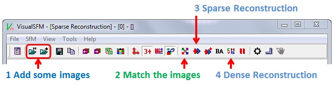
In Step 4, click (or shift+click) on the button to start dense reconstruction. In the popped up window, name your file and click ‘Save’. Since we do not change ‘Save as type’ options, this by default creates a new folder ‘yourfilename.nvm.cmvs’. The process may take several hours, depending on the number of images and features.
The Meshlab software will take on from here. See the Meshlab sections for details.
Meshlab
How to clean up point cloud in Meshlab?
Use  to select unwanted area. You can also use
  to select points on a plane. This is useful to remove points inside the model. For example, the interior of a car.
Press Shift to subtract selections (deselect). Press Ctrl to add selections (not very easy to control with plane selection mode, helpful in normal selection).
After selecting, click on the button again to stop selection mode. This is to be able to rotate the model and check, before removing the points. Click  to remove the selected area. Repeat until this layer is cleaned up.
How to prepare mesh for 3d printing in Meshlab?
The file required by the 3d printer has to be stl format, 1000kb or less.
In Meshlab, use Quadric Edge Collapse Decimation to simplify a mesh. Refer to: this article for more information.
From the menu, select Filters > Remeshing, simplification and construction > Quadratic Edge Collapse Detection. If your model is textured, there is also an option (with texture)
1) The target number of faces should be proportional to your desired file size. For example, a 190000-faces file has a size of 9000kb. So, the target number of faces should be around 20000, in order to get the size 9 times down. In most cases, a 20000-faces model will be around 1000bk.
2) Make sure to check the boxes for: Preserve Normal, Preserve Topology, Optimal position of qsimplified vertices, Planar simplification, Post-simplification cleaning
3) As usual, go to File > Export mesh as… Save it into .stl
How to import ASCII ply file into Meshlab?
When importing, a window appears and ask for:
- number of lines in header: (16 in our case)
- separation: (choose ; or . or space)
- separation columns: x y z r g b nx ny nz reflectance (refer to the header, and find the right one that matches the parameter order in the header).
Open the ASCII ply file in a text editor. Replace #QNAN with 0.
Replace all period sign with comma, if ERROR:unespect eof happens. It may be because of localization issues.
Check your data if part of the information failed to display (e.g. color of a certain part). The program omits invalid data and doesn’t always report error.
How to do measurement in Meshlab?
Filter > Normals, Curetures, and Orientations > transform scale
Press crtl+H to bring the image back to window.
How to align and merge (with poisson filter) point clouds in Meshlab?
Load the two meshes we wanted to align. Click on the Align button  . Select the main mesh layer, and set as Glue Here Mesh. Select on the to-be-aligned layer, and click Point Based Glueing.
Select four points to align the two mesh. (check the box on the left buttom to enable scaling.)
Click Ok when we finished selecting the aligning points. Check the result. Redo the alignment until we get satisfying result.
Go to Filter > Mesh Layer > Flatten Visible Layers. Now we should have one combined mesh out of the aligned ones. Go to Filter > Remeshing, Simplification and Reconstruction > Surface Reconstruction: Poisson. Give the proper octree value and divide solver. Wait for it to process. Save it as AlignedMesh.ply.
Open a new Meshlab workplace, load the raster files of the original main mesh layer (Open project…). Then import AlignedMesh.ply(Import mesh…). Now delete the point cloud model.
Go to Filters > Textures > Parameterization, texturing from registered rasters. Select the textrue png file of BOTH main mesh and to-be-aligned mesh.
Save the work.
Tips when merging a detailed denser mesh to a less dense one:
Since one of the two point clouds is not dense enough to conduct aligning. In this case, try to increase octree number to get denser mesh. Practically,
1) Take more pictures at proper intervals, and do the reconstruction again.
2) Chop off the less important part of the main (large) point cloud data; so that there’s enough memory for a denser mesh.
How to do mesh reconstruction in Meshlab?
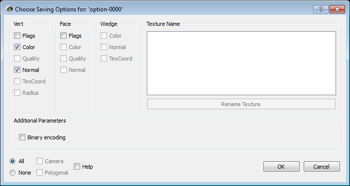
Note: When working in Meshlab, save  your work after each step as a different file. This secures any previous editing. This also prevents Meshlab crash due to memory allocation. When saving your work, always check the box for Color, Normal. We recommend to uncheck the box for Binary encoding. This will save all the information in ascii.
1. open the file and import the right mesh file from VisualSFM result
Open Meshlab, File > open project > browse to the folder (yourfilename).nvm.cmvs > 00, double click to open the bundle.rd.out file, then double click to open list.txt file. Wait for a few seconds to allow the mesh load.
Click on  button on the toolbar, if the Layer Dialog is not visible by default. Delete the current mesh (by right click on the name from the Layer Dialog on the right).
Go to File > Import Mesh… > navigate to 00/models. Press ‘ctrl’ on the keyboard, and select all ‘option-xxxx.ply’ files. Click open to import. There are more ply files like ‘option-0000.ply’, ‘option-0001.ply’, ‘option-0002.ply’, etc. Load them all.
2. Combine all the option-xxxx.ply files in Meshlab.
Note: this is optional. It makes the later on clean-up easier. But the color may not be rendered after this step.
From the menu, Filters> Mesh layer > flatten visible layers. Check all four boxes.
Save it.
3. Clean up the mesh.
To get a good mesh reconstruction, we need to unwanted points from the main scene/object:
- Surroundings that are not part of the scene/object
- Detached points scattered around the scene/object
- Noise
In the Layer Dialog, click to select the layer you would like to clean up. The selected layer will be highlighted.

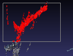
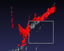
In the toolbar, click the Select Vertexes button. Left click and drag in the data displayed. The selected parts turn red. Press ‘ctrl’ and drag to add more to the selected; ‘shift’ and drag to remove from the selected. After selecting, click on the button again to stop selection mode. This is to be able to rotate the model and check, before removing the points.
Click to remove the selected area.
Repeat until this layer is cleaned up.
Save it either to the original mesh (by simply clicking the save button), or as a new mesh file by using file> export mesh as...
Note: In Meshlab, it’s very important that the layer is saved after every step. Otherwise, the program may crash due to memory overflow.
Select (highlight) another layer and repeat the process. Until all unwanted feature points are cleaned out.
4. Adjust and compute normal.
Note: this is optional. Skip this step the first time working with the results from VisualSFM, since VisualSFM output should already have normal information in it. Try to adjust and compute normals only when the reconstruction result is poor due to normal miscomputation.
In order to get correct normal vertexes for each side, you can cut the model into several pieces. Cut it in a way that points on each piece require relatively similar normals. When cutting, try to make sure there are common area on adjacent pieces, so that these pieces can be merged together layer. Compute normals for each piece.
Go to Render > show vertex normal, and also show arix. Go to Filters > Point set > Compute normals for point sets. Adjust the viewpoint position until the surface is properly recognized (most normal vertexes pointing upwards away from the object surface). Check the Flip normals w.r.t. viewpoint.
After each piece got the right normals. Use align function in Meshlab to merge the pieces back together.
5. Poisson reconstruction.
From the menu, go to Filter > Point sets > Surface Reconstruction: Poisson. Set the parameters (12, 10, 2, 1). Apply. Wait for the process to finish. A new poisson mesh layer will be created.
Note:
The parameters (12,10,2,1) is for optimal result. Reduce the numbers, e.g. (6,6,2,1), would save computational time and compromise the reconstruction quality.
The Poisson surfacing algorithm tends to produce bubble-like objects. You can remove the extraneous faces with “Filters > Selection > Select faces with edges longer than”. The default value will usually remove most extraneous faces.
6. Export the poisson mesh.
In the Layer Dialog, select/highlight the poisson mesh layer. Save it to the same folder as the option-xxxx.ply files. Save the project as well.
Delete the previous cloud point layers if necessary.
7. Clean up the mesh using selection and delete (refer to 3. Clean up the mesh). Save it .
8. Remove manifold Edges; manifold vertices.
Go to Filters > Selection > Select non Manifold Edges, and hit delete button. Save it .
Go to Filters > Selection > Select non Manifold Vertices, and hit delete button. Save it .
9. Create the textured mesh.
Filters > texture > Parameterization + texturing from registered raster... Set texture size as 4096 to get better results. The default texture map is named as ‘texture.png’. Check the boxes to use distance weight, use image border weight, and use UV stretching (optional). Hit Apply. Wait for it to complete. The completion message is delivered in the right bottom log window.
After completion, select the layer. Go to File> Export Mesh… Save it as mesh_textured.ply, in order to differentiate from the previous poisson mesh (no texture). It has to be saved in the same directory of the texture.png file. So, it’s safe to save everything in (yourfilename).nvm.cmvs\00\models.
The parameter 4096 can be replace with 2048 or 1024. Again, this speeds up the process and compromise the result.
10. Create the colored mesh.
Filter > Camera > Project active rasters color to current mesh, filling the texture. Rename the texture file, pixel size as 4096 (again, as 2048 or 1024 alternatively). Check the boxes to use angle weight, distance weight, image border weighter, and depth decontribute weight. Apply.
Save the layer as mesh_colored.ply; save the project as well. Go to file > reload the layer. Enable the texture render mode (the right most button). Switch to the Smooth view (second right most button) to see the color.
CloudCompare
How to visualize scanned point cloud in Cloudcompare?
In case the point cloud doesn’t come with color information. This may help to render the point cloud.
Select the layer.
Edit > Color > height Ramp
Maybe assign the color along y axis (or x axis, or z axis). Try it out to find best view.
How to measure distance/ accuracy of two point clouds?
1) Load the two point cloud layers.
2) Press Ctrl key on the keyboard, and select both layers. Now you need to cut the two layers into exact same size. Click on  ’segment’ tool from the tool bar. Click to set the start point, click again to set another point. When you finish setting the boundary, right click to release the cursor. In the segment menu bar, choose
  to keep the inner part of the polygon and accept the changes by clicking
  .
.
3) Press Ctrl key to select the new segmented layers. On the tool bar, click the button  for ‘compare cloud/cloud distance’. In the pompt-up window, see if the parameters on each tab are proper. We normally keep the ‘General parameters’ at the default value.
We can change the functions we want to use under ‘Local modeling’ tab. When no local model is used, the cloud to cloud distance is simply the nearest neighbor distance (using a kind of Hausdorff distance algorithm). If the reference cloud has a low density or has big holes, we use local modeling. All 3 models are based on the least-square best fitting plane that goes through the nearest point and its neighbors:
- Least squares plane: we use this plane directly to compute distances
- 2D1/2 triangulation: we use the projection of the points on the plane to compute Delaunay's triangulation (but we use the original 3D points as vertices for the mesh so as to get a 2.5D mesh).
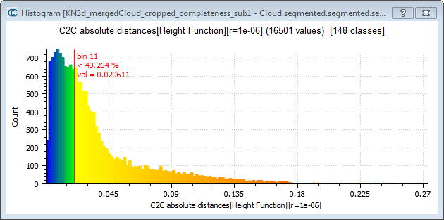
- Height function: the name is misleading but it is kept for consistency with the old versions. In fact the corresponding model is a quadratic function (6 parameters: Z = a.X2 + b.X + c.XY + d.Y + e.Y2 + f). In this case we only use the plane normal to choose the right dimension for 'Z'.
cite: http://www.cloudcompare.org/doc/wiki/index.php?title=Cloud-to-Cloud_Distance
4) On the third tab, click Compute to get the result.
5) You can view the histogram by clicking the
 ‘Show histogram’ button in the tool bar.
6) Save your segmented layers.
How to use the histogram in CloudCompare?
Use  to show more statistical results.
Scroll the mouse to increase/decrease the bin size. Drag the bar left/right to see statistics for different bins. This is very helpful to get the ideal bin size/ value you want.
More info: http://www.cloudcompare.org/doc/wiki/index.php?title=How_to_compare_two_3D_entities
CMPMVS
How to customize parameters in CMPMVS?
You can add more options to change parameters.
For example, copy the directory of mnv.ini file. Then put another single space, and paste the options you want. The options can be found in readme file under CMPMVS root folder.
Hit Enter to run CMPMVS with your settings.
The command line example:
C:\user\...\cmpmvs\CMPMVS_6>CMPMVS.exe E:\...\00\mvs.ini DoGenerateVideo=FALSE.