Workload imbalance is one of the major problems in training long-context Large Language Model (LLM) models. Long-context capability — the ability of a model to process and reason over hundreds of thousands of tokens at once — is critical for applications such as repository-level code understanding and multi-document reasoning. However, enabling long contexts makes the imbalance problem far more severe because the core attention computation grows quadratically with sequence length.

Imbalance among data parallel (DP) and pipeline parallel (PP) workers introduces stragglers or bubbles that cause severe slowdown. The problem becomes more severe as we scale to longer context lengths — because the quadratic attention cost amplifies any workload disparity — or to more GPUs, where even small per-device imbalances compound into large aggregate waste.

We believe that one of the major reasons for this slowdown is that the core attention , i.e., the $\text{softmax}(QK^{T})V$ kernel, colocates with the other linear parts. We argue that by disaggregating the quadratic part of the core attention computation from the linear part of the rest, we can fundamentally eliminate the imbalance and achieve near-linear scaling for long-context LLM training.

In this blog post, we first show why imbalance is a fundamental problem in the current wave of long-context LLM training, and then show how our technique, Core Attention Disaggregation (CAD) , can fundamentally eliminate imbalance across different GPUs — whether they are data-parallel workers or pipeline-parallel stages — without introducing extra overhead. As illustrated in our experimental results below, our prototype system DistCA achieves up to 1.35x speedup over state-of-the-art training systems.

Why is imbalance a fundamental problem of long-context LLM training?

Long-context LLMs have become the norm and the backbone of many modern applications, from coding assistants to agents that need to reason over entire repositories or databases. Yet, training these long-context models remains extremely costly. Compared to short-to-mid-context pretraining (e.g., 32K tokens), extending the context to 256K or 1M+ increases the core attention computation — the $\text{softmax}(QK^{T})V$ kernel — quadratically with sequence length. This quadratic growth causes severe imbalance across different GPU devices and training parallelism strategies.

Empirically, this imbalance has emerged as one of the major bottlenecks in today’s LLM training. Meta Llama-3 training on 128K experienced a 1.44x slowdown because of imbalance across GPUs, and others estimated a 2-4x slowdown when training models with 256K context length. Given that large-scale LLM training often spans weeks or months, this inefficiency substantially increases total training cost.

To understand this imbalance, let’s dive deeper and revisit what happens during LLM training.

LLM architecture and core attention (CA)

Figure 1 shows the structure of a typical LLM layer, and Figure 2 clarifies our terminology regarding core attention. Unlike most prior work, we use the term core attention (CA) to refer specifically to the computation that occurs after the QKV projection and before the O projection — the part implemented by kernels such as FlashAttention.

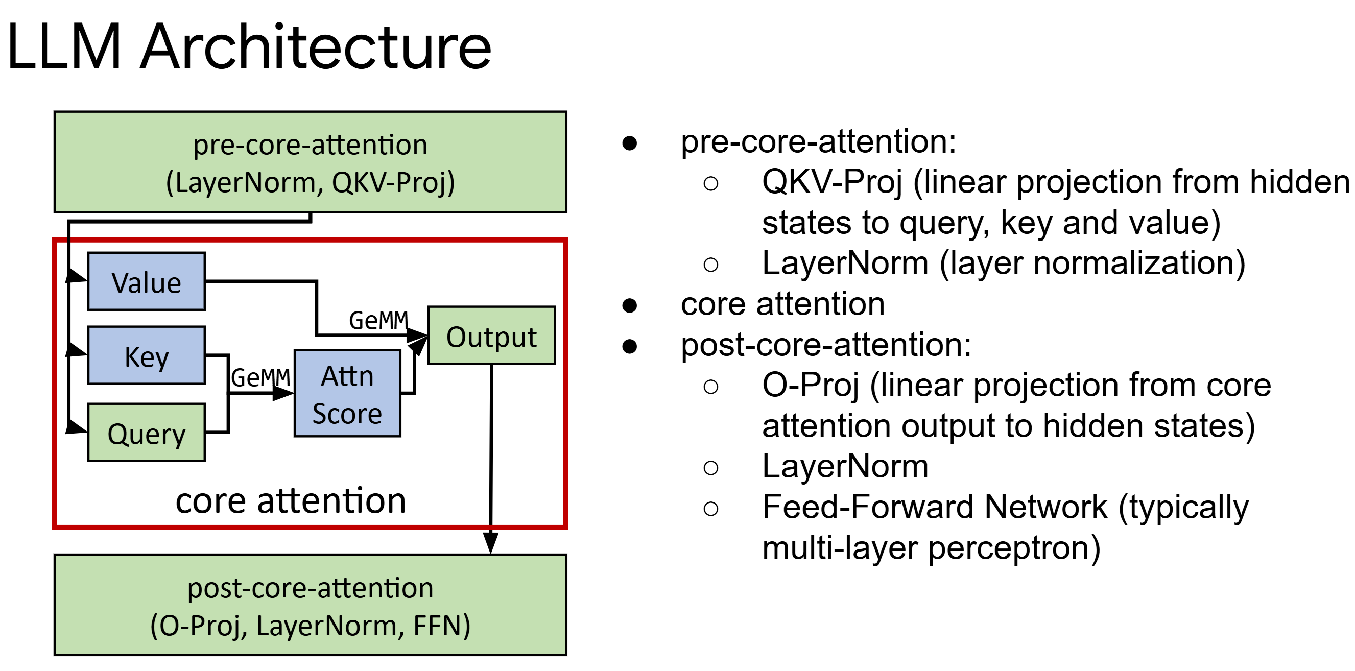
Figure 1. A typical LLM model within a layer.

Core attention (CA) contains only the $O(n^{2})$ computational component — the $\text{softmax}(QK^{T})V$ kernel — and nothing else. This distinction matters because, as we will show, the quadratic cost of CA is the root cause of workload imbalance, whereas all other parts of a layer scale linearly with the number of tokens.

In the standard literature, “attention” typically includes the QKVO projections (which are linear operations) as well as the quadratic kernel. We deliberately separate them: core attention refers only to the quadratic part, while the linear projections and FFN are grouped into pre-core-attention (pre-CA) and post-core-attention (post-CA) components. Isolating the quadratic component in this way is what allows us to disaggregate and rebalance it independently.

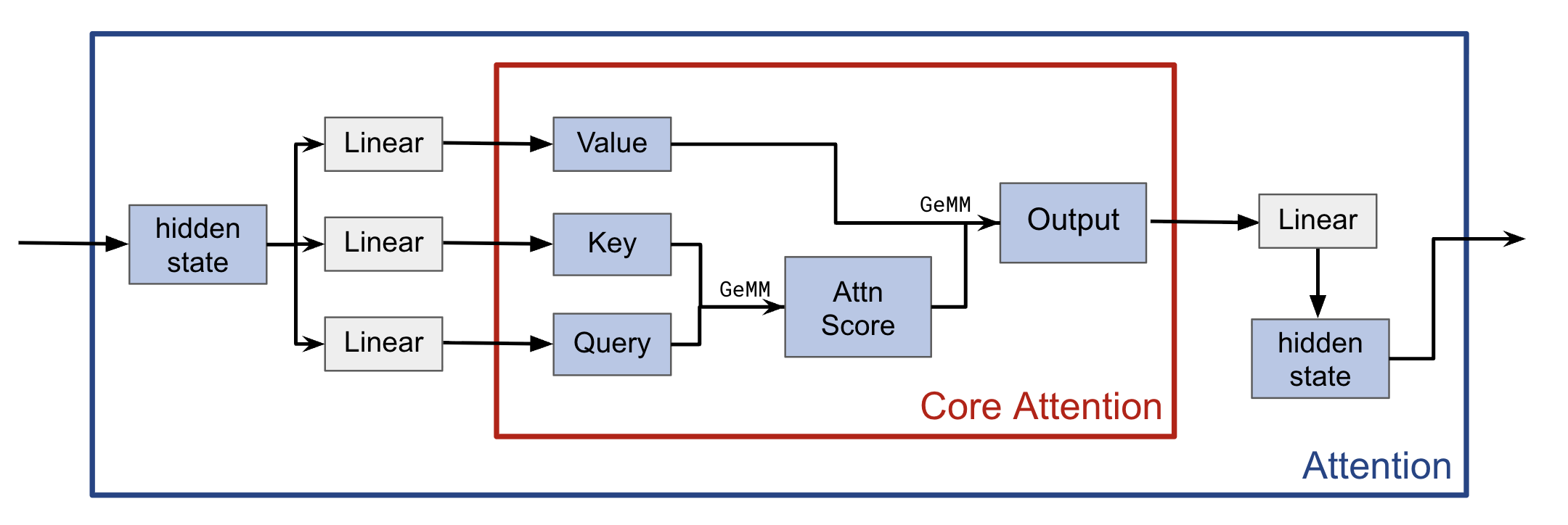
Figure 2. definition of core attention. core attention (CA) only contains the $O(n^{2})$ computational component, whereas the attention includes the QKVO projection (the linear computation components) and the $O(n^{2})$ core attention computation.

The fundamental source of imbalance is that core attention — with its quadratic complexity — is forced to run on the same device as the linear components. Because training documents vary in length, some devices end up with far more core attention work than others, as we explain next.

Document Packing

Documents come in variable lengths. To ensure efficiency, modern LLM training systems use document packing that packs the documents into batches such that each batch has the same length but contains multiple documents. As illustrated in Figure 3, packing eliminates the wasted padding tokens that would otherwise be needed to fill each batch to a uniform length. By removing this padding, every token processed by the GPU contributes to actual training, which saves memory and increases compute utilization.

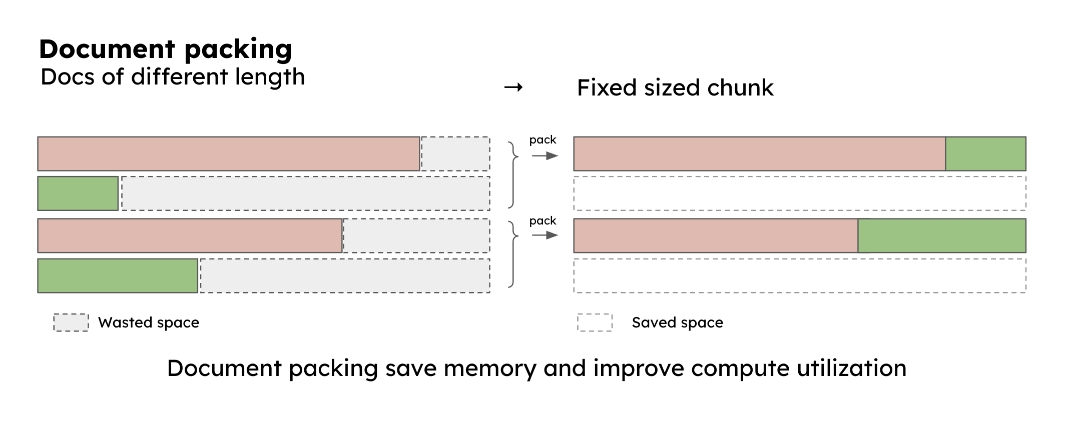
Figure 3. Document packing vs. non-document packing. Document packing packs the documents into batches such that each batch has the same length but contains multiple documents.

However, document packing introduces imbalance in the core attention operation. Figure 4 illustrates why with a concrete example. Suppose we have two batches, each containing the same total number of tokens (128K). Batch A holds a single 128K document, while Batch B holds eight 16K documents. Because core attention is quadratic, the cost for Batch A is proportional to $128K^2$, whereas the cost for Batch B is $8 \times 16K^2 = 8 \times (128K/8)^2 = 128K^2 / 8$ — only one-eighth of Batch A’s cost. In other words, Batch A takes 8x longer than Batch B to finish core attention, even though both batches have the same number of tokens. Crucially, this imbalance comes entirely from core attention: the linear components (projections, FFN) process the same number of tokens in both batches and are therefore perfectly balanced.

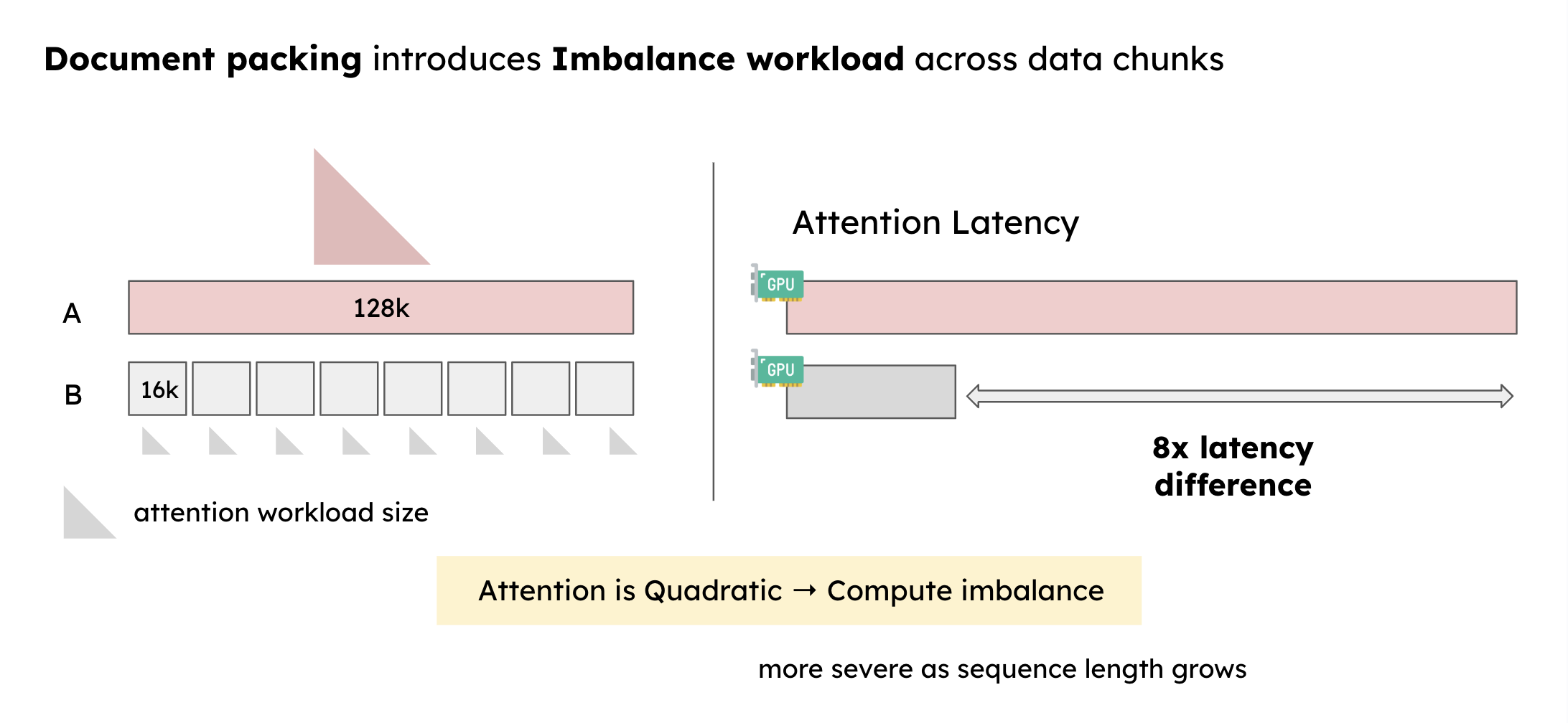
Figure 4. Document packing introduces imbalance in the attention operation across different batches.

Even worse, the imbalance grows as we push to longer contexts or more GPUs. Longer contexts increase the maximum possible disparity between a long document and a collection of short ones (since the quadratic gap widens with sequence length), while adding more GPUs means more batches, increasing the chance that at least one batch is significantly more expensive than the rest. Next, we explain how different parallelism strategies interact with this imbalance.

Parallelism Strategy in Distributed LLM Training Systems

Designing the right parallelism strategy is crucial for large-scale distributed LLM training. The most common approach is 4D parallelism, which combines Tensor Parallel (TP), Pipeline Parallel (PP), Data Parallel (DP), and Context Parallel (CP). In practice, a substantial amount of effort is spent tuning these parallelism dimensions, yet inefficiencies such as stragglers and pipeline bubbles often persist. We found that blindly scaling DP, PP, or CP will amplify the imbalance and make overhead dominant very quickly.

Data parallel introduces stragglers when DP ranks process microbatches with uneven core attention workload (and the same total token length). In DP, a training iteration has an optimizer step that synchronizes the gradients (all-reduce) from all ranks. When different DP ranks process microbatches with uneven core attention workload, the latency of the optimizer step is bound by the slowest worker (with the most core attention workload within its microbatch).

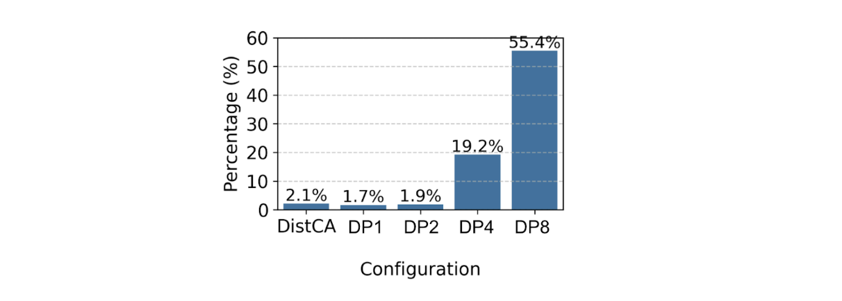
Figure 5a. total percentage of time that GPUs are unutilized because of stragglers as a proxy to measure the aggregate waste of GPU hours.

Figure 5a shows that data parallel introduces stragglers when data-parallel ranks process microbatches with uneven core attention workload. The number grows very quickly from ~2% in DP2 to an astounding 55% in DP8, as a direct result of stragglers in the DP rank with more attention computation.

Pipeline parallel further amplifies the imbalance problem. In PP, microbatches with uneven CA computation propagate along the pipeline, causing cascading amplification of the latency. Figure 5b shows such an example in a simple 1F1B schedule: when one microbatch (microbatch #1) has a much heavier computation, it affects the later microbatch schedule and introduces much more severe pipeline bubbles across stages. Techniques such as variable-length sharding try to mitigate this by moving documents from a compute-heavy batch into lighter ones. However, this approach invites significant memory imbalance across the microbatches and cannot mitigate imbalance across pipeline-parallel stages. This shows that naively scaling data parallelism or pipeline parallelism will make the imbalance more pronounced.

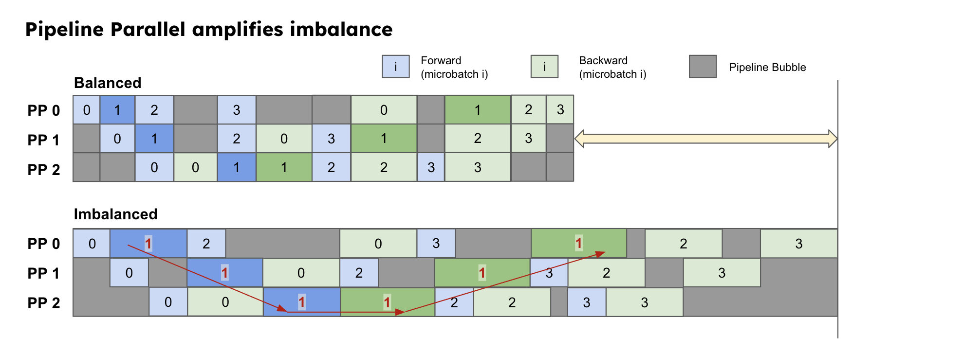
Figure 5b. Pipeline parallel amplifies the imbalance of core attention workload across different pipeline stages.

As an alternative, Context parallel (and variants such as per-doc context parallel sharding*(2)) shards each document (q-tensor) across context parallel workers in a way that has equal FLOPS. However, to compute the CA, each q-tensor shard also needs to have its associated KV tensors. This means context parallel must also all-gather the KV tensors across all GPUs — a communication step whose latency can quickly become dominant.

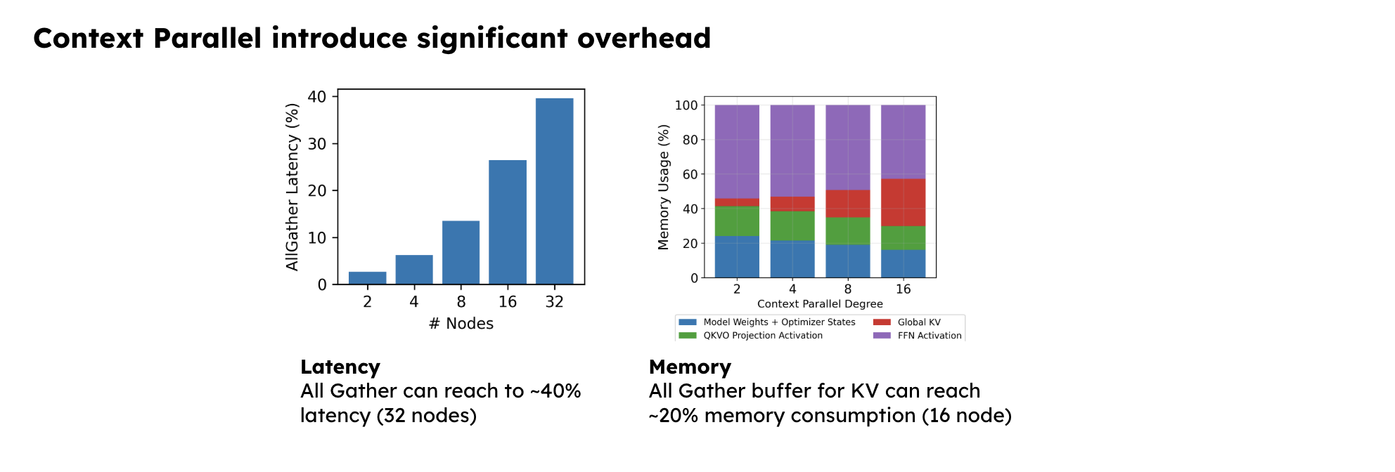
Figure 5c. Context parallel introduces overhead of all-gather as we scale the context parallel degree.

Figure 5c shows that as we scale CP degree, the latency of all-gather increases from 2% (CP2) of the total latency to 50% (CP32). Worse, the memory consumption of all-gather also increases significantly — from just <5% (CP2) of total memory to ~20% (CP16) just for storing the global KV tensors. Therefore, naively scaling CP will introduce a significant compute and memory overhead that prohibits further scaling.

In summary, we believe the fundamental limitation of current parallelism strategies in long-context training is colocation: colocating core attention and other linear components will always introduce compute or memory overhead that is hard to mitigate. This motivates us to disaggregate core attention from other components to fundamentally address the imbalance problem.

---

Existing systems that mitigate imbalance

Existing systems that try to mitigate the imbalance of CA mostly fall into two categories: variable-length data chunking and per-document context parallel sharding.

1. Variable-length data chunk

To mitigate CA imbalance, one natural way of thinking is to swap some documents from the more compute-heavy batch to the less compute-heavy one. As illustrated in Figure 6a, we swap 4x 16k documents from batch A to batch B to mitigate the imbalance between batch A and B.

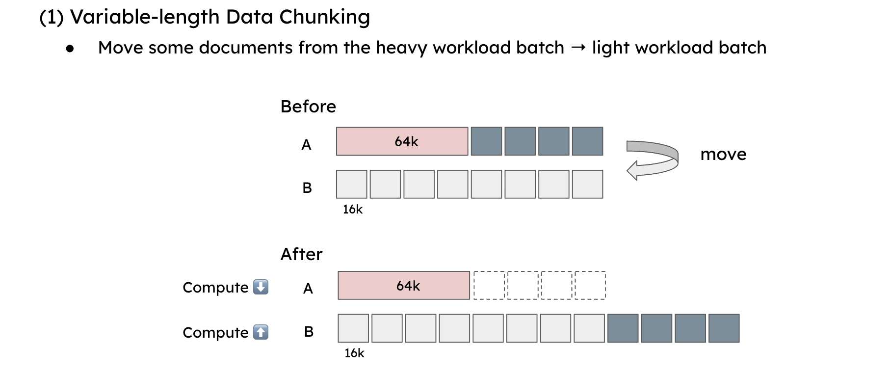
Figure 6a. Variable-length data chunking moves documents from the more compute-heavy batch to the less compute-heavy one to mitigate the imbalance between batch A and B.

But this method has many serious drawbacks. (1) It causes memory imbalance between batches. In this example, after moving the data chunks, B requires 3x the memory compared to A. The memory divergence can easily go up to 1.2x across 8 nodes, and grow even more as data parallel scales. (2) As sequence length grows, the GPU memory becomes much easier to saturate, and therefore simply moving documents around will fail to fully equalize attention compute due to these memory constraints.

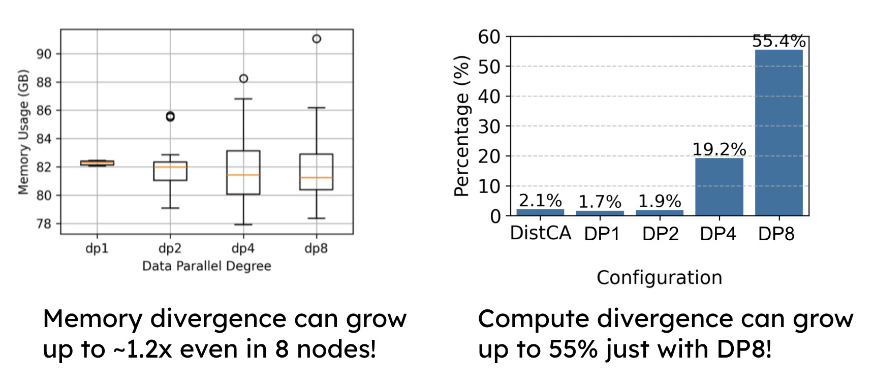
Figure 6b. Variable-length data chunking causes memory imbalance and compute underutilization as we scale the data parallel degree.

Figure 6b shows that compute underutilization can quickly go from just 2% in DP2 to up to 55% in DP8. As context length increases, variable-length data chunking will not be able to mitigate the imbalance of core attention anymore.

2. Per-document context parallelism

Another way to mitigate CA imbalance is to use per-document context parallelism (proposed in WLB-LLM). Essentially, as shown in Figure 7a, for each batch, we take each document and split it into CP shards (head-tail sharding) such that they have exactly the same computational workload. At data loading, we reorganize the tokens; and then at each layer forward, after producing the QKV in each CP rank, we perform an all-gather to gather all the KVs for the Q in this rank, and then perform core attention.

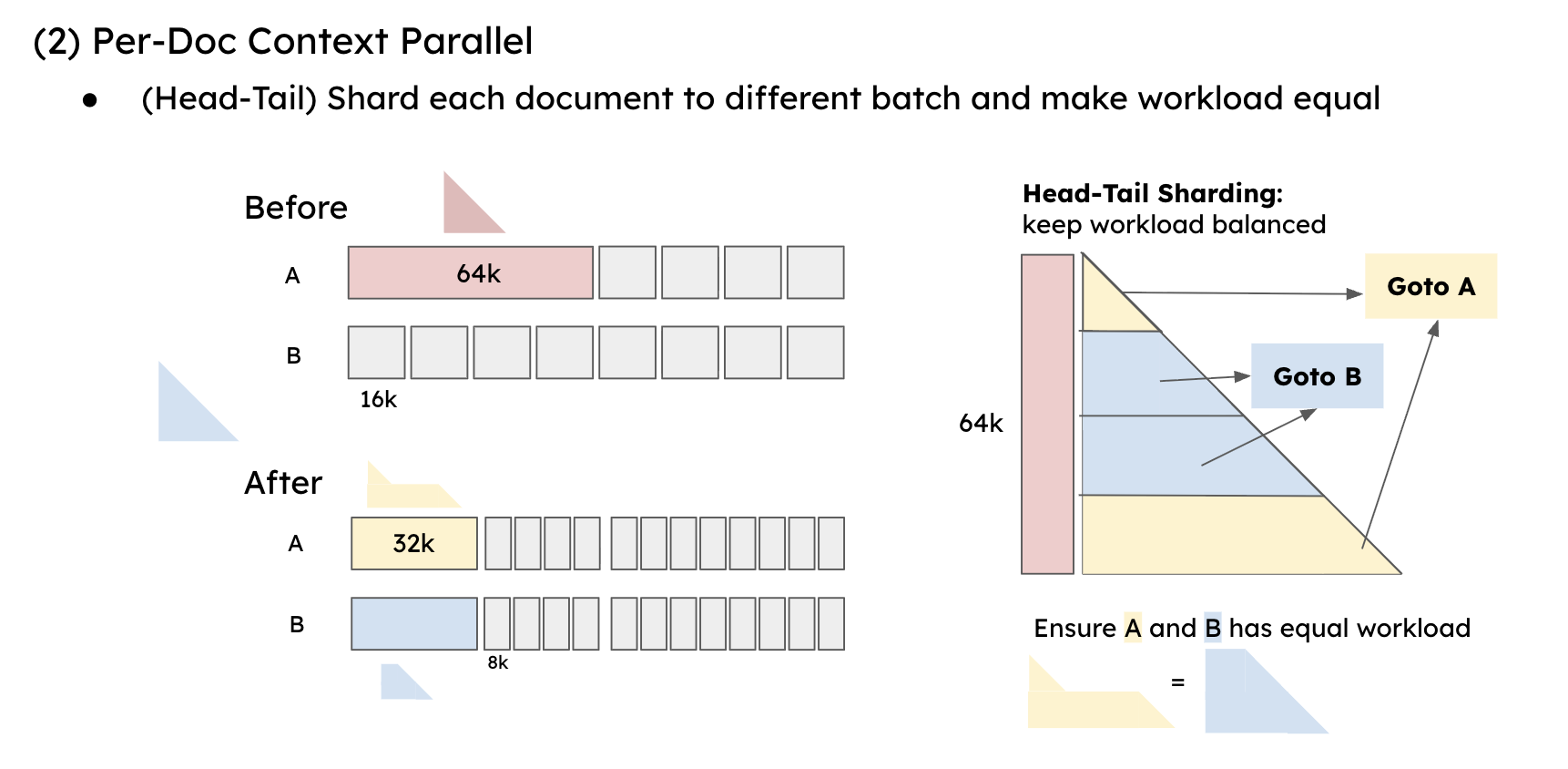
Figure 7a. Per-document context parallelism shards each document into CP shards such that they have the same computational workload.

However, per-doc CP also has two major drawbacks. First, assuming CP is placed across nodes, the all-gather operation does not scale well when the CP group grows larger. Figure 7b shows that the all-gather overhead can quickly rise to around 40% when $CP=32$. At the same time, the memory consumption used for all-gather grows from just 2% for $CP=2$ to almost ~20% at $CP=16$. These bottlenecks fundamentally limit the scalability of per-document CP.

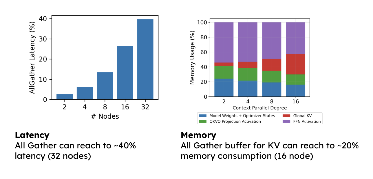
Figure 7b. Per-document context parallelism introduces overhead of all-gather as we scale the context parallel degree.

Existing training systems in academic work including WLB-LLM, FlexSP, and Zeppelin use a combination of these techniques. However, they still suffer from the same fundamental problems: they either invite memory imbalance across different ranks or introduce extra network and memory overhead. CAD fundamentally eliminates these problems and shows strong performance when scaling to longer context and larger scale.

---

CAD: Core Attention Disaggregation

The solution is simple: disaggregate CA from the rest of the model and treat CA as an individual unit of work (attention task) to be independently scheduled. This makes balancing core attention a much easier task without the need to care about the memory and compute overhead introduced by having linear components.

In other words, when CA (which has quadratic computational complexity) and the remaining components (which have linear complexity) are tied together, finding a balanced workload means to satisfy both $$\forall i\forall j:\sum_{d\in D_i} len(d)^2 = \sum_{d\in D_j} len(d)^2$$ and $$\forall i\forall j:\sum_{d\in D_i} len(d) = \sum_{d\in D_j} len(d)$$ here $D_i$ means the set of documents placed on GPU i, and $len(d)$ is the number of tokens for document $d$. The first equation is to guarantee that CA computation is evenly distributed onto each GPU, while the second is to balance other components of the model.

The set ${D_i | i \in \text{all GPUs}}$ provides all information about how documents are computed on a cluster of GPUs. We call this a document layout of a batch. Once disaggregated, CA and other components can have independent document layout. The layout for CA only needs to satisfy the first equation, while the layout for other components simply addresses the second. In addition to this, we will show that a single document’s CA computation can be further divided to smaller, independent units, making the workload balance of CA computation easy to reach.

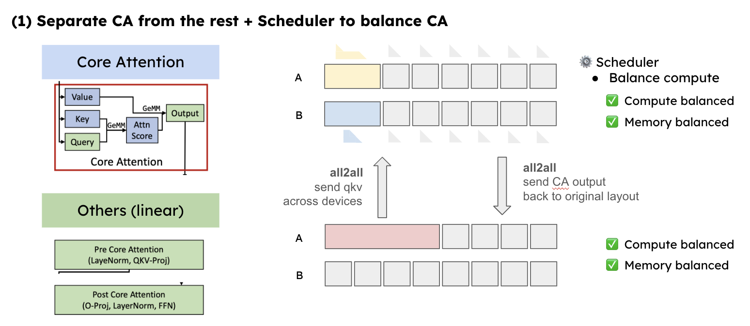
Figure 8. DistCA architecture. DistCA disaggregates core attention from other components and treats core attention as an individual unit of work (attention task) to be independently scheduled.

Figure 8 shows such an architecture. Once disaggregated, we can balance the core attention computation as individual units while maintaining the original document placement for other components of the model.

At first glance, disaggregation seems to introduce some additional overheads: (1) it introduces extra scheduling overhead to balance CA tasks on each device, and (2) when a document’s CA computation and other components’ computation are on different devices, the data will be moved between the two devices. We show that these problems can be solved by leveraging a few interesting compute and communication characteristics.

1/ The CA kernel can be divided and recombined almost arbitrarily

In modern attention kernels (e.g., FlashAttention), each GPU thread block is assigned a tile of the core attention computation. Each tile independently computes the attention output of a shard of the Query tensor with a shard of the Key and Value tensors, i.e. the $\text{softmax}(Q_iK_j^{T})V_j$, where $Q_i,K_j,V_j$ means a shard of $Q$, $K$, and $V$. The attention kernel can sustain high MFU (Model FLOPs Utilization) on variable-length fused document shards, provided each shard’s size is larger than this tile. As shown in Figure 9, if each CA shard’s length reaches tile size (128), the CA kernel throughput will be near peak throughput.

This means that a document’s CA computation can be arbitrarily sharded, and shards from multiple documents can be recombined into a single high-occupancy CA kernel without hurting kernel efficiency. As a result, a simple solution to balance CA computation is to:

1. compute the average computation workload on each GPU as a target FLOPs;
2. for each GPU, find documents whose CA computation is yet not allocated. Place a subset of these documents to that GPU until the total workload has reached the target.
3. When the GPU’s current workload is near the target FLOPs, and adding a whole document makes total FLOPs exceed the target: we can always find a shard whose FLOPs equals the remainder FLOPs. The rest of this document will be placed to the next GPU.

As a result, there are multiple document layouts satisfying the workload-balance constraint. We design algorithms that choose layouts with low communication overhead; the details are in our paper.

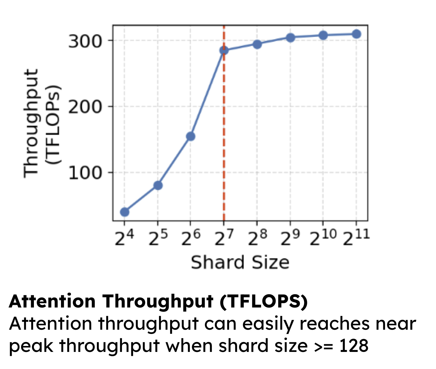
Figure 9. CA kernel throughput is near peak throughput when each CA shard length reaches 128.

2/ Core attention communication cost can be much lower than context parallel

Sending core attention input/output to/from the attention server seems to introduce more overhead compared to context parallel. But we observe the opposite: in context parallel, each document is sharded to all devices, and an all-gather collects all documents’ Key and Value tensors from all other devices. In CAD, instead, documents are sharded only when placing the entire document on a single device would push its FLOPs above the target described in the previous paragraph. As a result, the Key and Value tensors do not need to be broadcast to all devices, giving CAD significantly lower total communication volume and better scalability.

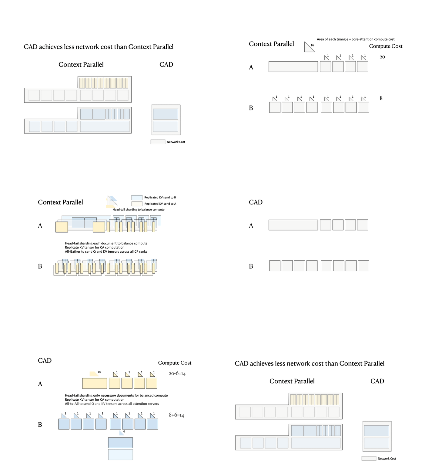
Figure 10. CAD can shard the long document and only move the shard large enough to achieve compute balance across different batches, making network communication much lower compared to context parallel.

3/ Ping-pong pipelining can hide communication almost entirely

One may have observed that despite the smaller volume of communication, CAD still introduces two communications for each layer in the forward (and backward) passes, and this additional synchronization may seem to offset the communication savings. Fortunately, LLM training typically uses large batch sizes to maximize throughput, and this enables us to use ping-pong pipelining to overlap communication with computation, thereby eliminating the additional all-to-all communication overhead.

As Figure 11 shows, we take a multiple of 2 microbatches (mb) every iteration, and at the end of a stage of the first mb (e.g., Pre.0), we take the second mb to run its computation (Pre.1) and launch the network communication for the output of Pre.0. In practice, as we scale to larger context length, the latency of computation will become large enough to overlap with communication. Therefore, using ping-pong parallel can effectively hide the communication overhead.

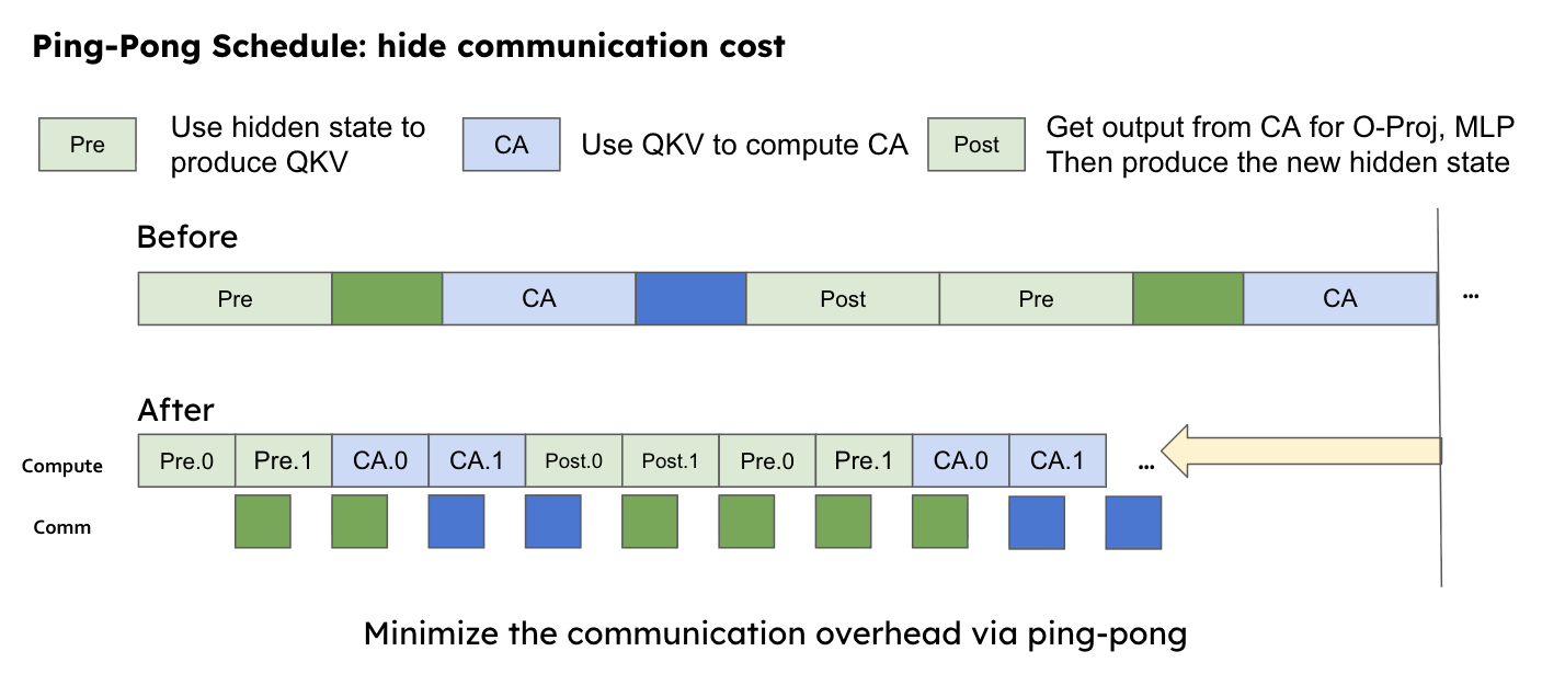
Figure 11. Ping-pong parallel can effectively hide the communication overhead.

4/ Imbalanced attention tasks can move across pipeline-parallel stages for balanced computation

Another major advantage of CAD is that GPUs from different pipeline-parallel (PP) ranks can now jointly balance core attention (CA) workloads. With CAD, we can design PP to alternate cleanly between CA and non-CA components. Since CA operates without weight parameters, its computation can be dynamically dispatched to GPUs in other PP ranks, thereby balancing the computation across PP stages.

As shown in Figure 12a (micro-view), within one forward layer, CAD can dispatch CA workloads to (1) idle GPUs in different PP ranks, or (2) rebalance CA tasks to different PP ranks. As shown in Figure 12b (macro-view), we remove most pipeline bubbles in pipeline parallelism without incurring extra overhead. Note that this is hard to do in conventional pipeline parallel schedules, because workload dispatch is confined within each stage, preventing cross-stage coordination. As the pipeline becomes deeper, this imbalance between microbatches amplifies even more and makes pipeline bubbles become increasingly difficult to eliminate.

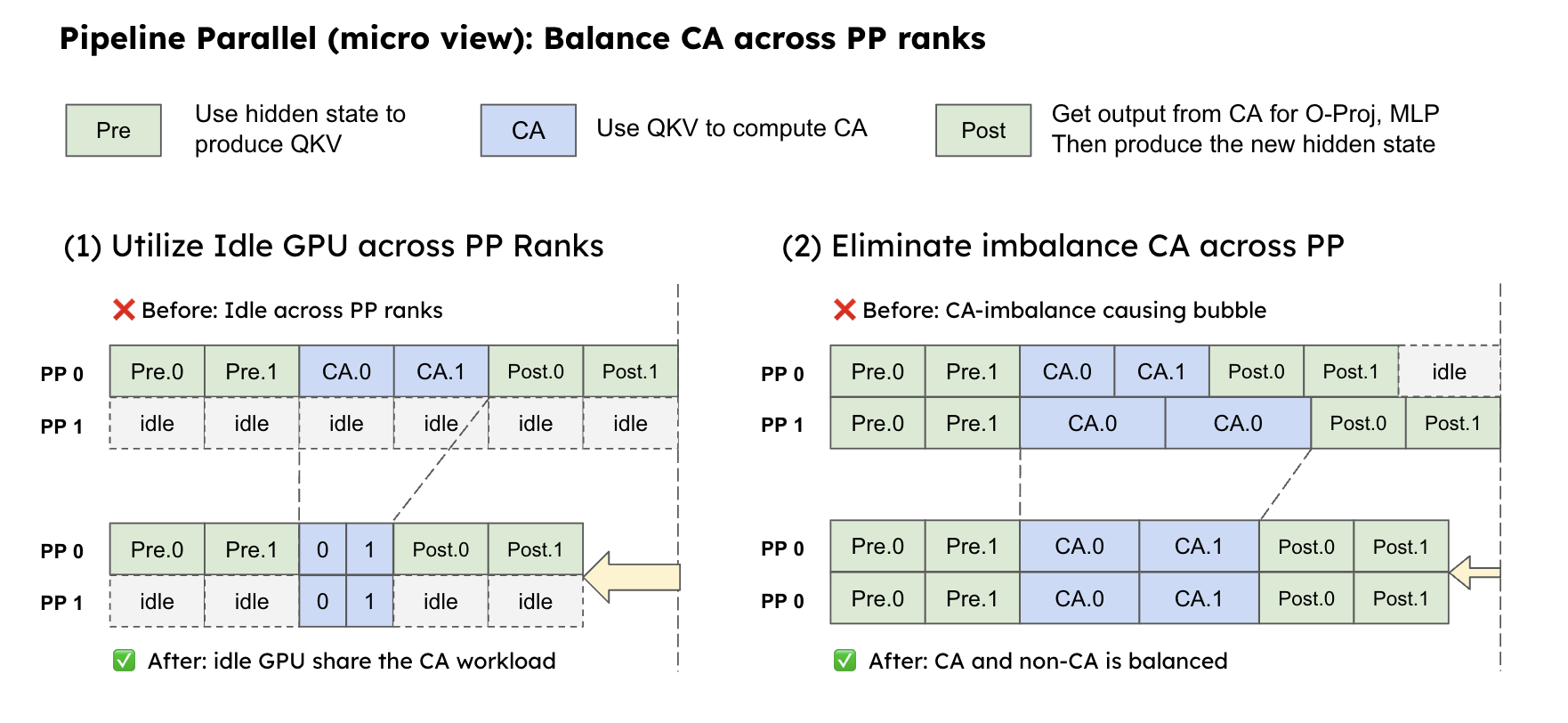
Figure 12a. CAD can dispatch CA workloads to idle GPUs in different PP ranks, or rebalance CA tasks to different PP ranks.

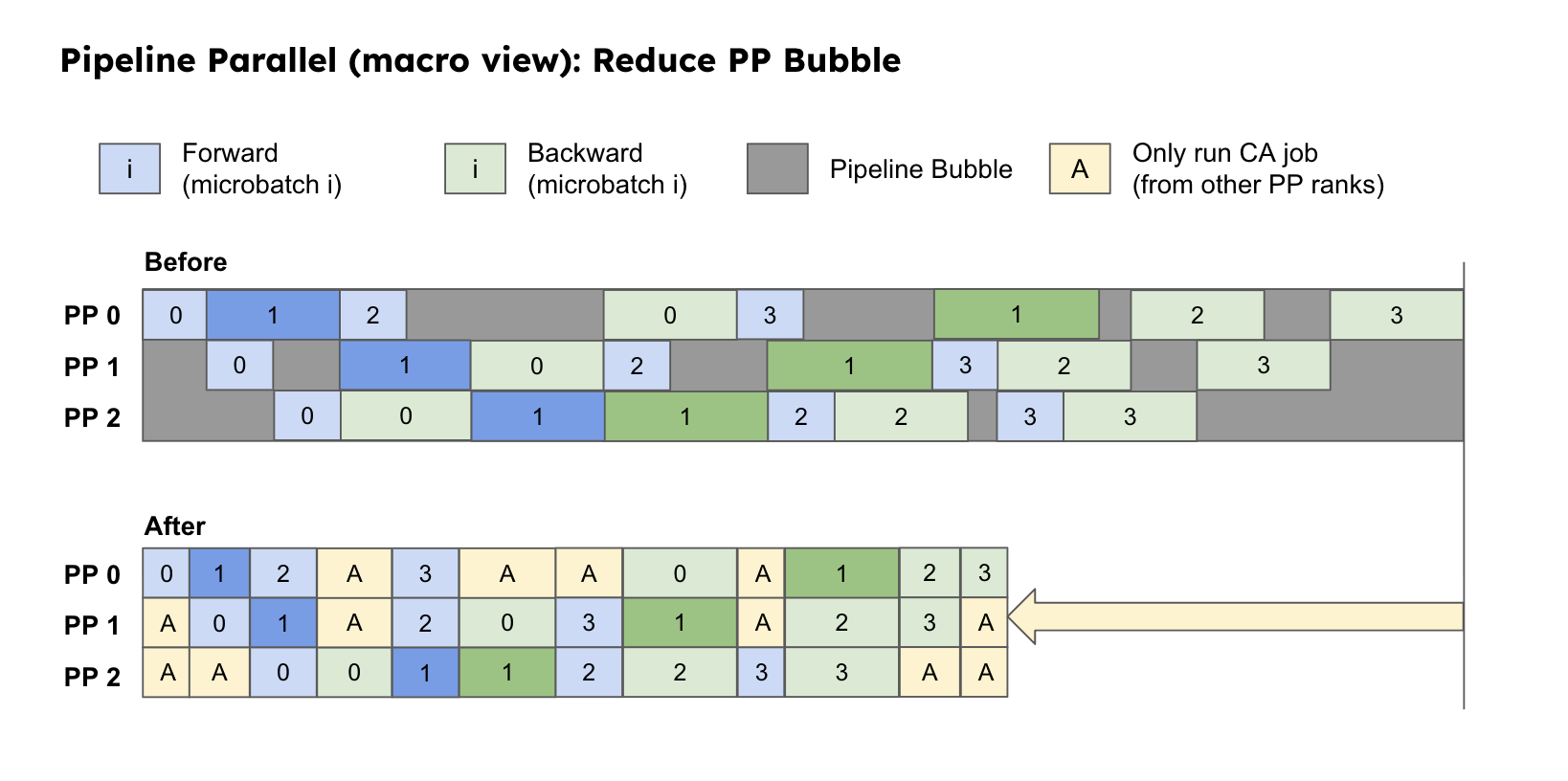
Figure 12b. CAD can remove most pipeline bubbles in pipeline parallelism without incurring extra overhead.

The CA divisibility property (1/) keeps scheduling cost low, while the lower communication volume (2/) and ping-pong pipelining (3/) hide communication cost, making CAD’s overhead near-zero. In addition, CAD opens a broader scheduling space that balances workloads not only across data-parallel ranks but also across pipeline-parallel stages (4/). Together, these properties make CAD a compelling approach for fundamentally eliminating imbalance in long-context LLM training.

We implement CAD in a system called DistCA , whose architecture and implementation we describe next.

---

DistCA: system design and evaluation of CAD

DistCA treats CAD as a first-class primitive in the LLM training system. It introduces the attention server , a new form of parallelism dedicated to handling core attention tasks. Since CA only depends on QKV tensors, an attention server does not need to hold any model weights for the computation, and is also stateless because neither the forward nor the backward pass needs to store any state in it.

At each iteration (Figure 13), the DistCA scheduler designs the optimal plan to shard and distribute CA tasks to attention servers. Each worker first runs the pre-core-attention (Pre-CA) modules, and then dispatches the QKV tensors according to the scheduler plan to the attention server via all-to-all communication. After the attention tasks are all done, the attention server sends the CA outputs back to the original layout and continues to run the post-core-attention parts. The DistCA runtime manages the model forward logic, network dispatch for CA tasks, and uses ping-pong parallel to overlap network communication with computation.

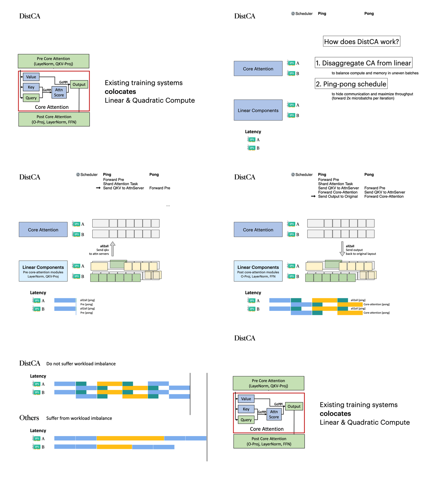
Figure 13. DistCA architecture and how it works.

One challenge is that assigning the attention servers into a dedicated pool of GPUs wastes a lot of memory and also underutilizes GPUs. To solve this, DistCA makes each GPU time-share between the CA and non-CA phases: each GPU alternates between the role of an attention server and a normal worker. This maintains high memory and compute utilization and balanced computation across devices.

We implement DistCA on top of Megatron-LM. We evaluate it on synthetic distributions and a real dataset (Prolong), using two model sizes (Llama-8B and Llama-34B), context lengths up to 512K, and up to 512 H200 GPUs connected by 400 Gbps InfiniBand. DistCA delivers up to 1.35x end-to-end throughput improvement, eliminates data-parallel and pipeline-parallel stragglers, and maintains near-perfect workload balance while fully hiding CAD’s communication overhead.

---

DistCA today and future work

Disaggregating core attention fundamentally eliminates the imbalance in large-scale LLM training systems. Our DistCA system efficiently rebalances CA workloads across devices, leverages ping-pong pipelining to hide communication overhead, and employs in-place attention servers to maximize GPU utilization. Together, it achieves both higher throughput and better scalability without architectural changes to the model.

Looking ahead, we believe CAD represents just the beginning of a broader disaggregation trend in training systems. Disaggregation opens the door to treating each component as an independent service — and even to leveraging heterogeneous hardware, tailoring each phase for better utilization and lower cost while maintaining high throughput.