HW 3 Solutions

CARNEGIE MELLON UNIVERSITY

15-826 - Multimedia databases and data mining

Spring 2007

[SOLUTIONS] Homework 3 - Due: Tuesday April 24, 1:30pm, in class.

For further questions or clarifications, please contact the TA.

Q1: 1-D DFT [10 pts]

Apply DFT to following datasets.

DS1: A noisy sine wave.
[1 pt] The time-plot (value vs time) of the original dataset,
[5 pt] The amplitude-frequency ("amplitude spectrum") plot for DFT.
[2 pt] What can you say given these plots, e.g. how many strong frequencies are there?
One strong frequency (but notice the symmetry/reflection over .5)
[1 pt] Give the sum of squares of the time values.
520.7175
[1 pt] Give the sum of squares of the amplitudes.
5.3321e+005 C.f. Parseval's theorem: "where X[k] is the DFT of x[n], both of length N." Note that Matlab does not do the normalization by N for you, so you must normalize the numbers Matlab gives you in order to see Parseval's equivalence: sum of squares of the time values = (1/# samples) * sum of squares of the amplitudes in this case: 520.7175 = 1/1024 * 5.3321e+005
DS2: A different noisy sine wave.
[1 pt] The time-plot (value vs time) of the original dataset,
[5 pt] The amplitude-frequency ("amplitude spectrum") plot for DFT.
[2 pt] What can you say given these plots, e.g. how many strong frequencies are there?
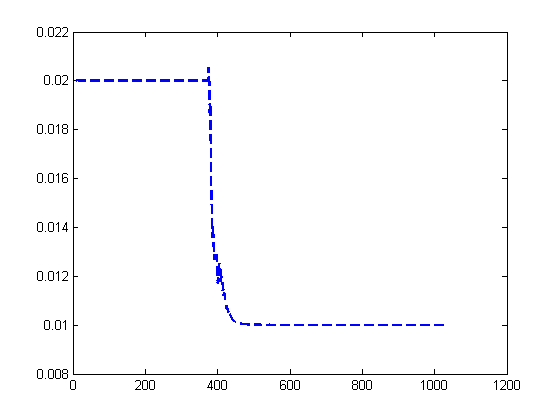
One strong frequency, and another strong, but weaker one.
[1 pt] Give the sum of squares of the time values.
1.7409e+004
[1 pt] Give the sum of squares of the amplitudes.
1.7827e+007
DS3: White noise.
[1 pt] The time-plot (value vs time) of the original dataset,
[5 pt] The amplitude-frequency ("amplitude spectrum") plot for DFT.
[2 pt] What can you say given these plots, e.g. how many strong frequencies are there?
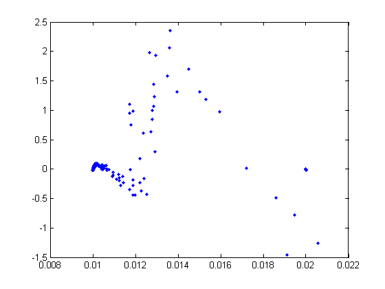
No strong frequency stands out -- just noise
[1 pt] Give the sum of squares of the time values.
350.7012
[1 pt] Give the sum of squares of the amplitudes.
3.5912e+005

Q2: 1-D DWT [10 pts]

Apply DWT using Haar wavelets (code available here) and DFT to this simulated heart beat.

What to hand in:

[1 pt] The time-plot of the original dataset,
[1 pt] The amplitude-frequency ("amplitude spectrum") plot for DFT.
1. [1 pt] What can you say given these plots?
2. There seem to be a mixture of a few strong, regular frequencies of varying strength.
[2 pt] Plot the scalogram for DWT as a set of histograms (1 per scale).
The top line of each plot shows the original signal. This plot shows the approximate coefficients for each scale 1 through 9: While this plot again shows the original signal on top, followed by the detail coefficients for scales 1 through 9:
1. [1 pt] What can you say given these plots? Any dominant frequencies? Any spikes?
2. There are a few dominant frequencies, but no real spikes.
[1 pt] The time plot of the reconstructed version using only the top 5 DFT coefficients
1. [1 pt] Give the root mean squared error (RMSE) between this reconstructed version and the original.
2. If we don't count the symmetric coefficients twice, we can exactly recreate the signal using only 5 dft coefficients, and thus have zero RMSE.
[1 pt] Give the time plot of the reconstructed version using only the top DOF DWT coefficients
1. [1 pt] The root mean squared error (RMSE) between this reconstructed version and the original:
2. Wavelets are not as good at compressing this kind of periodic signal, and so we get a higher RMSE of .2165 (though the difference is hard to see in the plot). The exact value will depend on which coefficients you chose, but should be higher than the value for the DFT reconstruction.

Q3: 2D DFT and DWT [10 pts]

Download this 2D black and white image of 16*16 pixels, each with intensity 0 or 1. The origin of the image (x=1, y=1) is in the top left corner (like a matrix). The format for the data is "x y value" where value is the black-white intensity (0 = black, 1 = white).

Hand in the following:

[2 pt] The 2-d image of the dataset,
[2 pt] Draw the 2-d grey-scale image of the reconstructed version using only the top 3 DFT coefficients as defined in Q2 above. The degrees of freedom (DOF) should be about 6.
Again, your exact image will depend on the coefficients you used. One common mistake here was to only do the transform on one dimension of the iamge (x-, or y-axis) leaving you with a reconstruction that looked "stripey" instead of "blocky."
1. [2 pt] What is the root mean squared error (RMSE) between this reconstructed version and the original, where RMSE is defined as before, but this time averaging over all pixels (ie, all values of i and j):
  Using this formula: and the top 3 real coefficients, the RMSE is .2288. Again, your RMSE may vary (depending on if you used a different DFT formula, or a different number of DOF), but should be significantly higher than the one you get using DWT (since, for this signal, wavelets are more suited for compression than fourier). In general, nicely periodic signals will be compressed more efficiently by DFT, while signals with big discontinuities will do better with DWT.
[2 pt] Draw the reconstructed version using only the top DOF DWT coefficients
Your results may vary, but the reconstruction using dwt should look better than dft.
1. [2 pt] What is the root mean squared error (RMSE) between this reconstructed version and the original?
2. Using the above formula and reconstruction, the RMSE is .1849. Again, your numbers may vary, but RMSE should be lower than with DFT (even zero, depending on which coefficients you chose).

Q4: Iterated Function Systems [15 pts]

Dragon Curve

Write code to generate and plot the following curve for any order n:

(Figure 1)

Please submit:
1. [3 pts] The plot of the curve at order 6 (your code should generate a set of 2-d line segments, which you can plot using your favorite utility, eg, gnuplot, xgraph, etc)
3. [2 pts] The fractal dimension of the curve in the limit (as n goes to infinity)
4. The fractal dimension for iterated function systems can be calculated as fractal dimension = log(# resulting shapes after split)/log(magnification) For this shape, each single line becomes two lines, so the numerator is 2, and each resulting line is the hypotenuse of a right triangle of base 1/2, so the magnification is sqrt(2), so we get fractal dimension = log(2)/log(sqrt(2)), so the fractal dimension is 2.
5. [2 pts] Your code
6. Code may vary, but in general should produce output like this
X-shape

Get the IFS code here. Now use it to plot the following X-shape.

(Figure 2)

Please submit:
1. [2 pts] The plot of 1,000 points that you generated using Barnsley's IFS algorithm (in the ifs code)
2. Depends on your sample, but should look something like this.
3. [2 pts] The fractal dimension of the x-shape
4. Using the formula from before, we have: log(5)/log(3) ~ 1.465
5. [2 pts] The correlation integral (distance vs # pairs) of your 1,000 points
6. Depends on your sample, but should be near the exapected value of log(5)/log(3)
7. [2 pts] Your code (ie, the parts of the IFS code that you modified. Eg, input.parms)
8. Modify your transformation matrix to look something like:
```
double a[]= {0.333, 0.333, 0.333, 0.333, 0.333};
double b[]= {0.0, 0.0, 0.0, 0.0, 0.0};
double c[]= {0.0, 0.0, 0.0, 0.0, 0.0};
double d[]= {0.333, 0.333, 0.333, 0.333, 0.333};
double e[]= {0.0, 0.667, 0.333, 0.0, 0.667 };
double f[]= {0.0, 0.0, 0.333, 0.667, 0.667 };
double p[]= {0.2, 0.2, 0.2, 0.2, 0.2};
```

Q5: SVD [10 pts]

Consider the following Document by Term matrix: DocTerm

Hand in:

[3 pts] The SVD components (the U, lambda, V matrices, specifying which is which).
The key thing to notice here is that all but the first three entries in the lambda matrix are effectively zero:
```
   lambda = [ 42.4   0.0  0.0
               0.0  21.2  0.0
               0.0   0.0  7.1]
```
[1 pts] Your estimate of the number of topics for the DocTerm dataset.
Based on the above analysis of the lambda matrix, estimate three topics.

[6 pts] For every topic, give a sorted list of documents (specified by row-id) that participate in this topic, along with their weight in the topic.





The key here was to recognize that each document only had weight in
one of the three topics. The clusters were:

   Topic 1 contains documents:
2     3     4     5     7     9    10    11    12    
16    19    22    23    25    26   30    31    33
34    35    36    37    38    39    41    42    44    
48    50    51    52    53    55    56    57    59    
60    62    63    68    69    70    71    72    73 
74    75    76    78    79    80    81    82    83    
88    90    91    94    96    99

Topic 2 contains documents:  
1     8    13    15    17    18    21    27    28    
29    32    43    45    47    49   54    58    61    
65    66    67    77      85    87    89    92    93    
95    97    98
                                                
Topic 3 contains documents:    
6    14    20    24    40    46    64    84    86   100

Q6: 3-D SVD [15 pts]

This dataset contains 10,000 points constructed in the following manner:

Points are sampled from a three dimensional (N=3) spherical (Sigma is now the 3x3 identity matrix) Gaussian centered at the origin (mu is now the vector: <0, 0, 0>).
1. The first coordinate of the sampled point is multiplied by a scalar a
2. The second coordinate of the sampled point is multiplied by a scalar b
3. The third coordinate of the sampled point is multiplied by a scalar c
These warped points are all finally rotated and translated by some unknown affine transformation (which is the same for all points).

[15 pts] Given this data, recover a, b and c.



The key was to realize the translation could be undone by first
subtracting the mean of each dimension away from each point, thus
recentering the points around the origin. You could then perform
SVD to recover the scales of: 21.5, 7.7, and 2.2. Exact results may
differ depending on how you do normalization.

Q7: Regression and Recursive Least Squares [30 pts]

Implement the method of Recursive Least Squares (RLS), with forgetting, from the paper by [Yi et al, ICDE 2000] ( pdf, ps.gz), or from [Chen & Roussopoulos, SIGMOD 94] ( pdf, ps.gz).
Apply the recursive least squares (RLS) algorithm to this simulated, fictitious dataset. We would like to identify a) when the patient began taking the medicine and b) what effect (if any) this medicine had on the relationship between the patient's calories, exercise and cholesterol. We also want to investigate how much of a difference running ordinary least squares (OLS, read more here or see property C1 in slide #17 in these slides, which is equivalent to equation 4 in this paper) and RLS makes on the results. At every week we estimate w1(t) and w2(t) that best fit the data up to and including week t.

What to hand in:

Plot both the time-series of how w1(t) and w2(t) change over time, and the 2-d scatter plot of <w1(t), w2(t)> over time t, as estimated by:
1. [4 pts] RLS with no forgetting (ie, lambda = 1)
2. W1 vs time:
  
  W2 vs time:
  
  W1 vs W2 (across time):
3. [4 pts] RLS with the forgetting factor lambda = 0.95
4. W1 vs time:
  
  W2 vs time:
  
  W1 vs W2 (across time):
5. [4 pts] OLS with no forgetting (ie, lambda = 1)
6. W1 vs time:
  
  W2 vs time:
  
  W1 vs W2 (across time):
7. [4 pts] OLS with the forgetting factor lambda = 0.95
8. W1 vs time:
  
  W2 vs time:
  
  W1 vs W2 (across time):
[2 pts] Based on these plots, when (which week) did the patient begin taking her medication?
The changes begin near week 375. This is most clear in the plots with forgetting.
[2 pts] Give the running times (wall clock) of each of the four experiments
The exact running times will depend on your machine and implementation details, but in general your OLS code should run at least an order of magnitude more SLOWLY than RLS. The main idea is to see that RLS can do almost as well as RLS in significantly shorter time. For example, on an Intel Dual Core 2Ghz machine running Windows XP, with 2 gb of ram: OLS takes 7.093 seconds while RLS takes only .078 seconds on the same machine (~100 times faster)
[10 pts] Submit your code for both RLS and OLS



RLS with and without forgetting: as in the 
paper



OLS without forgettig: Essentially, you do ordinary least squares
regression on subsets of the full dataset:

 Input: full data X and Y
 For each t in 0 to T
        X_t = X[0...t]
        Y_t = Y[0...t]
        W_t = inv(X_t’*X_t)*(X_t’)*Y_t;
 end

OLS with forgettig: Same as above, but this time you discount older observations (closer to t=0) with exponential decay alpha, as in RLS. This makes mistakes on older observations less costly:

 Input: full data X and Y and forgetting factor alpha
 For each t in 0 to T
        X_t = X[0...t]
        Y_t = Y[0...t]
        For each t_alpha in 0 to t
                L[t_alpha] = alpha^(t-t_alpha)
        end for
        W_t = inv((X_t’)*L*X_t)*(X_t’)*L*Y_t;
 end for