Deriving Complexity

       

There are two complexities associated with all computations in NESL.

1. Work complexity: this represents the total work done by the computation, that is to say, the amount of time that the computation would take if executed on a serial random access machine. The work complexity for most of the sequence functions is simply the size of one of its arguments. A complete list is given in Table 1. The size of an object is defined recursively: the size of a scalar value is 1, and the size of a sequence is the sum of the sizes of its elements plus 1.

2. Depth complexity: this represents the parallel depth of the computation, that is to say, the amount of time the computation would take on a machine with an unbounded number of processors. The depth complexity of all the sequence functions supplied by NESL is constant.

The work and depth complexities are based on the vector random access machine (VRAM) model [13], a strictly data-parallel abstraction of the parallel random access machine (PRAM) model [19]. Since the complexities are meant for determining asymptotic complexity, these complexities do not include constant factors. All the NESL functions, however, can be executed in a small number of machine instructions per element.

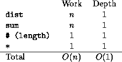
The complexities are combined using simple combining rules. Expressions are combined in the standard way--for both the work complexity and the depth complexity, the complexity of an expression is the sum of the complexities of the arguments plus the complexity of the call itself. For example, the complexities of the computation:

 sum(dist(7,n)) * #a  

can be calculated as:

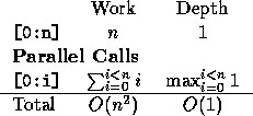
The apply-to-each construct is combined in the following way. The work complexity is the sum of the work complexity of the instantiations, and the depth complexity is the maximum over the depth complexities of the instantiations. If we denote the work required by an expression exp applied to some data a as , and the depth required as , these combining rules can be written as

 

 

where sum and max_val just take the sum and maximum of a sequence, respectively.

As an example, the complexities of the computation:

 {[0:i] : i in [0:n]}  

can be calculated as:

Once the work (W) and depth (D) complexities have been calculated in this way, the formula

 

places an upper bound on the asymptotic running time of an algorithm on the CRCW PRAM model (P is the number of processors). This formula can be derived from Brent's scheduling principle [14] as shown in [41, 13, 30]. The term shows up because of the cost of allocating tasks to processors, and the cost of implementing the sum and scan operations. On the scan-PRAM [6], where it is assumed that the scan operations are no more expensive than references to the shared-memory (they both require on a machine with bounded degree circuits), then the equation is:

 

In the mapping onto a PRAM, the only reason a concurrent-write capability is required is for implementing the <- (write) function, and the only reason a concurrent-read capability is required is for implementing the -> (read) function. Both of these functions allow repeated indices (``collisions'') and could therefore require concurrent access to a memory location. If an algorithm does not use these functions, or guarantees that there are no collisions when they are used, then the mapping can be implemented with a EREW PRAM. Out of the algorithms in this paper, the primes algorithm (Section 2.2) requires concurrent writes, and the string-searching algorithm (Section 2.1) requires concurrent reads. All the other algorithms can use an EREW PRAM.

As an example of how the work and depth complexities can be used, consider the kth_smallest algorithm described earlier (Figure 1). In this algorithm the work is the same as the time required by the standard serial version (loops have been replaced by parallel calls), which has an expected time of [18]. It is also not hard to show that the expected number of recursive calls is , since we expect to drop some fraction of the elements on each recursive call [37]. Since each recursive call requires a constant depth, we therefore have:

Using Equation 3 this gives us an expected case running time on a PRAM of:

One can similarly show for the quicksort algorithm given in Figure 2 that the work and depth complexities are and [37], which give a EREW PRAM running time of:

In the remainder of this paper we will only derive the work and depth complexities. The reader can plug these into Equation 3 or Equation 4 to get the PRAM running times.