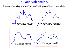
Figure 26: Cross validation checks how well a model generalizes to new data
Cross validation is a model evaluation method that is better than residuals. The problem with residual evaluations is that they do not give an indication of how well the learner will do when it is asked to make new predictions for data it has not already seen. One way to overcome this problem is to not use the entire data set when training a learner. Some of the data is removed before training begins. Then when training is done, the data that was removed can be used to test the performance of the learned model on ``new'' data. This is the basic idea for a whole class of model evaluation methods called cross validation.
The holdout method is the simplest kind of cross validation. The data set is separated into two sets, called the training set and the testing set. The function approximator fits a function using the training set only. Then the function approximator is asked to predict the output values for the data in the testing set (it has never seen these output values before). The errors it makes are accumulated as before to give the mean absolute test set error, which is used to evaluate the model. The advantage of this method is that it is usually preferable to the residual method and takes no longer to compute. However, its evaluation can have a high variance. The evaluation may depend heavily on which data points end up in the training set and which end up in the test set, and thus the evaluation may be significantly different depending on how the division is made.
K-fold cross validation is one way to improve over the holdout method. The data set is divided into k subsets, and the holdout method is repeated k times. Each time, one of the k subsets is used as the test set and the other k-1 subsets are put together to form a training set. Then the average error across all k trials is computed. The advantage of this method is that it matters less how the data gets divided. Every data point gets to be in a test set exactly once, and gets to be in a training set k-1 times. The variance of the resulting estimate is reduced as k is increased. The disadvantage of this method is that the training algorithm has to be rerun from scratch k times, which means it takes k times as much computation to make an evaluation. A variant of this method is to randomly divide the data into a test and training set k different times. The advantage of doing this is that you can independently choose how large each test set is and how many trials you average over.
Leave-one-out cross validation is K-fold cross validation taken to its logical extreme, with K equal to N, the number of data points in the set. That means that N separate times, the function approximator is trained on all the data except for one point and a prediction is made for that point. As before the average error is computed and used to evaluate the model. The evaluation given by leave-one-out cross validation error (LOO-XVE) is good, but at first pass it seems very expensive to compute. Fortunately, locally weighted learners can make LOO predictions just as easily as they make regular predictions. That means computing the LOO-XVE takes no more time than computing the residual error and it is a much better way to evaluate models. We will see shortly that Vizier relies heavily on LOO-XVE to choose its metacodes.

Figure 26: Cross validation checks how well a model generalizes to new data
Fig. 26 shows an example of cross validation performing better than residual error. The data set in the top two graphs is a simple underlying function with significant noise. Cross validation tells us that broad smoothing is best. The data set in the bottom two graphs is a complex underlying function with no noise. Cross validation tells us that very little smoothing is best for this data set.
Now we return to the question of choosing a good metacode for data set a1.mbl:
File -> Open -> a1.mbl
Edit -> Metacode -> A90:9
Model -> LOOPredict
Edit -> Metacode -> L90:9
Model -> LOOPredict
Edit -> Metacode -> L10:9
Model -> LOOPredict
LOOPredict goes through the entire data set and makes LOO predictions for each point. At the bottom of the page it shows the summary statistics including Mean LOO error, RMS LOO error, and information about the data point with the largest error. The mean absolute LOO-XVEs for the three metacodes given above (the same three used to generate the graphs in fig. 25), are 2.98, 1.23, and 1.80. Those values show that global linear regression is the best metacode of those three, which agrees with our intuitive feeling from looking at the plots in fig. 25. If you repeat the above operation on data set b1.mbl you'll get the values 4.83, 4.45, and 0.39, which also agrees with our observations.