
Algorithms for the Sum-check Protocol
How to Verify Private (or Expensive) Computations
Suppose a hospital runs a statistical analysis over millions of patient records to determine whether a drug is effective. The computation takes days of cluster time, and the raw data cannot be shared due to privacy regulations. A regulatory agency needs to trust the result—but cannot re-run the computation or inspect the data. How can they be confident the analysis was performed correctly?
This is an instance of a broader challenge: we increasingly rely on computational results we cannot feasibly re-check. Sometimes the data is private, so other parties cannot re-run the computation at all. Other times the data is public but the computation is simply too expensive to repeat.
Cryptographic zero-knowledge proof systems address this dilemma. They let an untrusted prover convince a verifier that some private data satisfies a public statement. For instance, you can prove that you are over 18 or that your account has sufficient balance without revealing your birthdate or financial history. Proofs are short and fast to verify—milliseconds rather than hours or days—so the savings compound when many parties need to check the same result.
Over the past decade, cryptographic proof systems have matured from theoretical curiosities into practical tools, with applications ranging from age verification [1] to blockchain scalability [2]. However, generating a proof is still orders of magnitude slower than running the computation natively, making prover efficiency a central challenge.
Many state-of-the-art proof systems owe much of their performance to a classical protocol from 1992: the sum-check protocol [4]. Sum-check’s very success, however, has made it a bottleneck: it often consumes the majority of the total proving time. In this blog post, I will introduce the sum-check protocol, detail well-known algorithms for its prover, and present a new technique that speeds up the prover in practical settings [9].
Sum-Check Protocol Overview
The sum-check protocol [4] is an interactive proof that allows an untrusted prover to convince a computationally limited verifier of the value of a very large sum. Informally, the verifier wants to check a sum of many evaluations of a multivariate polynomial over a large product domain, but would like to avoid explicitly computing all of those values.
We will require two properties from the protocol: completeness (an honest prover always convinces the verifier) and soundness (a cheating prover is caught with overwhelming probability). After describing the protocol, we will verify that sum-check satisfies both.
Formally, we fix a finite field \( \mathbb{F} \) (a number system with addition, subtraction, multiplication, and division, but only finitely many elements) and a multivariate polynomial \( p(X_1, \dots, X_n) \in \mathbb{F}[X_1,\dots, X_n] \), of degree bounded by \( d \) in each variable. The sum-check claim is then $$ \sum_{x_1 \in H_1, \dots, x_n \in H_n} p(x_1,\dots,x_n) = c, $$ for some evaluation domains \( H_1, \dots, H_n \subseteq \mathbb{F} \) and a claimed value \( c \in \mathbb{F} \). In most applications, and for the remainder of this blog post, we restrict the inputs to the Boolean hypercube , namely the domain \( H_1 = \dots = H_n = \{0,1\} \). The claimed value \( c \) remains an arbitrary element of \( \mathbb{F} \).
The verifier knows \( p \), or at least has query access to \( p \) (meaning it can ask for evaluations of \( p \) at chosen points), but wants to use this access as little as possible. Naively, the verifier could evaluate \( p \) on all \( 2^n \) points of \( \{0,1\}^n \) and sum the results, which takes work on the order of \( O(2^n) \). The key idea of sum-check is that, by interacting with an untrusted prover who supplies additional “auxiliary” polynomials, the verifier can reduce the work of checking the original claim to checking a related claim about \( p \) at a single randomly chosen point.
In particular, the data that the prover sends at each round are the “one-dimensional” slices of this multivariate polynomial. In the first round, the prover sends the univariate polynomial $$ s_1(X) = \sum_{(x_2,\dots,x_n) \in \{0,1\}^{n-1}} p(X, x_2,\dots,x_n). $$ If the original claim is correct, then \( s_1(X) \) has degree at most \( d \), and moreover \( s_1(0) + s_1(1) = c \). The verifier checks precisely these two conditions, and rejects if either fails.
If both checks pass, the verifier samples a random challenge \( r_1 \gets \mathbb{F} \) and sends it to the prover. This random point forces consistency: if the prover sent an incorrect low-degree \( s_1 \), then with high probability (at least \( 1 - d / \lvert \mathbb{F} \rvert \)) it disagrees with the honest slice at \( X=r_1 \). Over a sufficiently large field (e.g., at least 128-bit), this error probability is negligible. We discuss why this is the case under soundness below.
After this first round of interaction, the prover and verifier have effectively reduced the problem to showing that $$ \sum_{(x_2,\dots, x_n) \in \{0,1\}^{n-1}} p_1(x_2, \dots, x_n) = c_1, $$ where we define \( p_1(x_2,\dots,x_n) := p(r_1, x_2,\dots,x_n) \) and \( c_1 := s_1(r_1) \). That is, we have “bound” the first variable to \( r_1 \) (where “bound” here means “substituted in,” not lower or upper bound) and now reduce to a new sum-check instance in \( n-1 \) variables. The protocol then repeats the same pattern on this new instance: in the second round, the prover sends a univariate polynomial $$ s_2(X) = \sum_{(x_3,\dots,x_n) \in \{0,1\}^{n-2}} p_1(X, x_3,\dots,x_n), $$ the verifier again checks the degree and the equation \( s_2(0) + s_2(1) = c_1 \), samples a fresh random \( r_2 \gets \mathbb{F} \), sets the new claim \( c_2 := s_2(r_2) \), and continues.
After \( n \) rounds, all variables have been fixed to random challenges \( r_1,\dots,r_n \in \mathbb{F} \), and the verifier is left with a single claim of the form $$ p(r_1,\dots,r_n) = c_n $$ that it can check directly using its query access to \( p \).
What properties does the sum-check protocol satisfy? The first is completeness . If the original sum claim is correct and the prover follows the rules, then every round’s check passes, and at the end we really do have \( p(r_1,\dots,r_n) = c_n \), so the verifier accepts.
The more interesting property is soundness , which is about what happens when the original claim is false. In that case, no matter how a (possibly malicious) prover behaves, at some round it must send a polynomial that is not the “right” one. This is exactly the situation we previewed when introducing the random challenge \( r_1 \): by the Schwartz–Zippel lemma [5], two different degree-\( d \) polynomials over a field agree on at most a \( d / \lvert \mathbb{F}\rvert \) fraction of points, so a random challenge \( r_i \) catches the lie except with that probability. With a large field, this is negligible.
Brief Interlude on Multilinear Polynomials
So far, we have only described sum-check as a protocol on polynomials over finite fields. But how does this relate to any computation performed in the real world? The key bridge between the two is called the arithmetization of the computation: we first transform the computation trace—such as the values of all registers over time, or the sequence of memory accesses and intermediate constraint values—into polynomials, and then we use sum-check to reason about those polynomials instead of the original computation.
In many sum-check-based proof systems, the traces and constraint tables are represented as multilinear polynomials . A multilinear polynomial is a multivariate polynomial where each variable appears with degree at most \( 1 \). For instance, $$ q(X_1, X_2, X_3) = 3X_1 X_3 + 2X_2 + 5 $$ is multilinear, while \( X_1^2 + X_2 \) is not. A key fact is that a multilinear polynomial in \( n \) variables is uniquely determined by its values on the \( 2^n \) points of the Boolean hypercube \( \{0,1\}^n \). This gives a natural way to encode a length-\( 2^n \) vector as a multilinear polynomial: the polynomial’s values on the Boolean hypercube are exactly the entries of the vector.
We can also make this encoding precise with a mathematical formula. Given a function \( p : \{0,1\}^n \to \mathbb{F} \) (for example, a vector of trace or constraint values indexed by \( y \in \{0,1\}^n \)), its multilinear extension is the unique multilinear polynomial \( \widetilde{p}(X_1,\dots,X_n) \) that agrees with \( p \) on all Boolean points. The formula for the multilinear extension is as follows: $$ \widetilde{p}(X_1,\dots, X_n) = \sum_{y \in \{0,1\}^n} \widetilde{eq}(\vec{X}, y) \cdot p(y), $$ where the equality polynomial \( \widetilde{eq} \) is defined by $$ \widetilde{eq}(\vec{X}, \vec{Y}) = \prod_{i=1}^n \big((1 - X_i)(1 - Y_i) + X_i Y_i\big). $$ You can think of \( \widetilde{eq} \) as an indicator for equality on the Boolean hypercube: for any \( \vec{x}, \vec{y} \in \{0,1\}^n \), \( \widetilde{eq}(\vec{x}, \vec{y}) = 1 \) if \( \vec{x} = \vec{y} \) and \( 0 \) otherwise. Plugging this into the formula above, each term in the sum “picks out” \( p(y) \) at a single Boolean point.
As a concrete example, consider the vector \( [3, 1, 4, 2] \). We index its entries by the points of \( \{0,1\}^2 \): $$ p(0,0) = 3, \quad p(0,1) = 1, \quad p(1,0) = 4, \quad p(1,1) = 2. $$ Using the formula above, the multilinear extension is $$ \begin{aligned} \widetilde{p}(X_1, X_2) &= 3 \cdot (1 - X_1)(1 - X_2) + 1 \cdot (1 - X_1)X_2 + 4 \cdot X_1(1 - X_2) + 2 \cdot X_1 X_2 \\ &= 3 - 2X_2 + X_1 - X_1 X_2. \end{aligned}$$ You can verify that \( \widetilde{p} \) recovers the original vector on Boolean inputs. Moreover, the sum of the vector entries equals the sum of \( \widetilde{p} \) over the hypercube: $$ \sum_{(x_1, x_2) \in \{0,1\}^2} \widetilde{p}(x_1, x_2) = 3 + 1 + 4 + 2 = 10. $$ Verifying this sum is exactly a sum-check instance.
Example: Arithmetizing a Batched Zero-Check
Now that we have seen multilinear polynomials, let’s see how they allow us to turn common constraints into sum-check instances.
Consider a tiny 4-cycle execution trace of a program containing only two instructions, either add two numbers (think of them as field elements) or multiply two numbers:
| Cycle \( i \) | Instruction | \( x(i) \) | \( y(i) \) | \( z(i) \) |
|---|---|---|---|---|
| 0 | ADD | 3 | 5 | 8 |
| 1 | MUL | 2 | 6 | 12 |
| 2 | ADD | 1 | 4 | 5 |
| 3 | MUL | 7 | 3 | 21 |
Suppose we want to check that every ADD instruction was executed correctly. We introduce a selector column \( S_{\text{ADD}} = [1, 0, 1, 0] \), where a 1 marks an ADD row, and an error column $$ E = z - (x + y) = [0, 4, 0, 11]. $$ The constraint we want is $$ S_{\text{ADD}}(i) \cdot E(i) = 0 \quad \text{for all } i \in \{0, 1, 2, 3\}. $$ Concretely, the four products are $$ 1 \cdot 0 = 0, \quad 0 \cdot 4 = 0, \quad 1 \cdot 0 = 0, \quad 0 \cdot 11 = 0. $$ This is a batched zero-check : we have two columns whose element-wise product must vanish everywhere. In a real program execution, we typically need to check that thousands or millions of such per-row products are all zero, so it is essential to verify them as a single batched check rather than one row at a time.
To use sum-check, we index the four cycles by the Boolean hypercube \( \{0,1\}^2 \), say $$ (0,0) \leftrightarrow 0,\quad (0,1) \leftrightarrow 1,\quad (1,0) \leftrightarrow 2,\quad (1,1) \leftrightarrow 3. $$ Let \( p(X_1, X_2) \) and \( q(X_1, X_2) \) be the multilinear extensions of \( S_{\text{ADD}} \) and \( E \) respectively. In this example, we can even write them down explicitly: $$ p(X_1, X_2) = 1 - X_2, \qquad q(X_1, X_2) = 4X_2 + 7X_1 X_2. $$ Their product is $$ p(X_1, X_2) \cdot q(X_1, X_2) = X_2(1 - X_2)(4 + 7X_1), $$ which vanishes on every Boolean point because \( X_2(1 - X_2) = 0 \) whenever \( X_2 \in \{0,1\} \).
This pointwise condition can be bundled into a single sum over the hypercube. Define $$ g(x_1, x_2) = p(x_1, x_2) \cdot q(x_1, x_2), $$ and we want to demonstrate that \( g \) is zero everywhere on the Boolean hypercube. Equivalently, the multilinear extension \( \widetilde{g} \) is the zero polynomial on \( \{0,1\}^2 \). This in turn is equivalent to the polynomial identity $$ \sum_{(x_1, x_2) \in \{0,1\}^2} \widetilde{eq}\big((X_1, X_2), (x_1, x_2)\big) \cdot p(x_1, x_2) \cdot q(x_1, x_2) = 0. $$ We reduce this identity to a sum-check instance by sampling a random point \( (r_1, r_2) \in \mathbb{F}^2 \) and checking that it holds at that point: $$ \sum_{(x_1, x_2) \in \{0,1\}^2} \widetilde{eq}\big((r_1, r_2), (x_1, x_2)\big) \cdot p(x_1, x_2) \cdot q(x_1, x_2) = 0. $$ By the Schwartz–Zippel lemma, if this sum-check claim holds for random \( (r_1, r_2) \), then \( \widetilde{g} \) is zero everywhere on \( \{0,1\}^2 \), except with negligible probability \( 2 / \lvert \mathbb{F} \rvert \). So, instead of checking four separate products directly, we check a single polynomial identity at a random point. The same pattern scales to an arbitrary \( 2^n \)-row execution trace: each operation type contributes selector columns and low-degree constraint polynomials, and a full program execution becomes a large collection of such checks. This is the basic arithmetization step that lets proof systems handle general computation.
Existing Algorithms for Sum-Check
We now turn to prover algorithms. We will focus on the most common setting in modern proof systems: sum-check over a low-degree function applied to one or more multilinear polynomials. This captures many real applications, including the batched zero-check above. In the zero-check example, the sum involved an \( \widetilde{eq} \) factor alongside the product \( p \cdot q \); in practice, the \( \widetilde{eq} \) factor has special structure that can be exploited separately (we return to this point in the conclusion). For now, to simplify the exposition, we specialize to the case of a product of two multilinear polynomials $$ \sum_{x \in \{0,1\}^n} p(x) \cdot q(x) = c, $$ where \( p, q : \{0,1\}^n \to \mathbb{F} \) are given by their evaluations on the Boolean hypercube. The algorithms we cover straightforwardly generalize to the product of an arbitrary number of multilinear polynomials.
Linear-time algorithm
The first prover algorithm we consider, following Vu, Setty, Blumberg, and Walfish [6] and Thaler [7], runs in linear time in the number of summands \( N = 2^n \). This is the main setting in many proof systems: it proves statements (like a batched zero-check) with only a constant-factor overhead relative to the input size \( N \).
Recall that in the first round of sum-check, the prover needs to compute and send the univariate polynomial $$ s_1(X) = \sum_{(x_2,\dots,x_n) \in \{0,1\}^{n-1}} p(X, x_2,\dots,x_n) \cdot q(X, x_2,\dots,x_n). $$ Since \( s_1(X) \) has degree at most \( 2 \), it is determined by its values at any three points, say \( 0,1,2 \). The prover computes \( s_1(0), s_1(1), s_1(2) \) in a single pass over the \( 2^n \) evaluations of \( p \) and \( q \), using three accumulators initialized to zero. For each \( x’ = (x_2,\dots,x_n) \in \{0,1\}^{n-1} \), it looks up \( p \) and \( q \) at \( (0,x’) \) and \( (1,x’) \), and adds the corresponding contributions: $$ % \begin{cases} s_1(0) \mathrel{+}= p(0, x’) \cdot q(0, x’),\quad s_1(1) \mathrel{+}= p(1, x’) \cdot q(1, x’),\quad s_1(2) \mathrel{+}= p(2, x’) \cdot q(2, x’). % \end{cases} $$ In the above, we do not have explicit evaluations of \( p \) and \( q \) at \( (2, x’) \), but we can extrapolate them from the values at \( (0, x’) \) and \( (1, x’) \). This relies on the fact that \( p \) and \( q \) are multilinear, meaning each has degree at most \( 1 \) in its first variable. In other words, for a fixed \( x’ \), the map \( X_1 \mapsto p(X_1, x’) \) is a degree-1 (affine) polynomial \( a + b \cdot X_1 \), so $$ p(2, x’) = 2 \cdot p(1, x’) - p(0, x’), $$ and the same holds for \( q \). This gives us the formula $$ p(2, x’) \cdot q(2, x’) = (2 \cdot p(1, x’) - p(0, x’)) \cdot (2 \cdot q(1, x’) - q(0, x’)). $$
After the verifier sends a random challenge \( r_1 \), the prover needs the bound polynomials $$ p_{1}(x_2,\dots,x_n) := p(r_1, x_2,\dots,x_n), \quad q_{1}(x_2,\dots,x_n) := q(r_1, x_2,\dots,x_n) $$ in order to continue the protocol on \( n-1 \) variables. The linear-time algorithm explicitly computes and stores the evaluations of \( p_{1} \) and \( q_{1} \) on all \( 2^{n-1} \) points of \( \{0,1\}^{n-1} \). It does so by making another pass over the original evaluation tables \( (p(x))_{x \in \{0,1\}^n} \) and \( (q(x))_{x \in \{0,1\}^n} \) and computing, for each \( (x_2,\dots,x_n) \in \{0,1\}^{n-1} \), the bound evaluations via linear interpolation: $$ p_{1}(x_2,\dots,x_n) = (1 - r_1) \cdot p(0, x_2,\dots,x_n) + r_1 \cdot p(1, x_2,\dots,x_n),$$ $$q_{1}(x_2,\dots,x_n) = (1 - r_1) \cdot q(0, x_2,\dots,x_n) + r_1 \cdot q(1, x_2,\dots,x_n).$$ These new vectors of size \( 2^{n-1} \) serve as the “input data” for the next round: they play the same role that the original evaluation tables of \( p \) and \( q \) played in the first round, but for the reduced \( (n{-}1) \)-variable problem. In each subsequent round \( i = 2, 3, \dots, n \), the prover repeats the same pattern on these smaller vectors of evaluations to compute \( s_i \), then binds the next challenge \( r_i \) and shrinks the vectors of evaluations again, and so on.
Cost Analysis: In round \( i \), the prover performs \( O(2^{n-i}) \) field operations. Summing over rounds, the total work is linear in \( N = 2^n \): $$ O(2^n + 2^{n-1} + \dots + 1) = O(2^n). $$
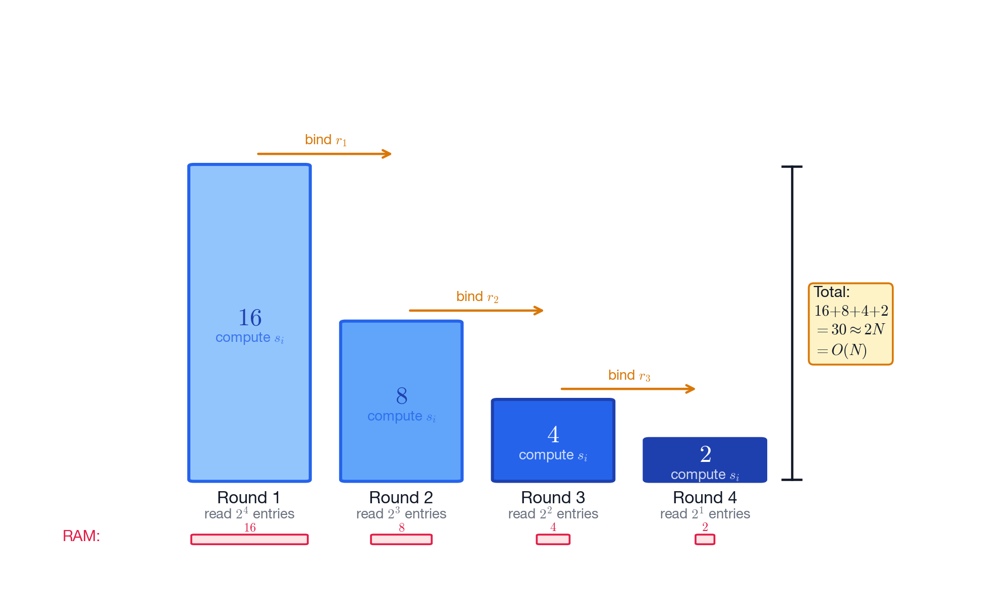
One downside of this algorithm is the need for linear storage: starting from round \( 2 \), the prover must store \( p_1 \) and \( q_1 \). This may be fine for small-to-medium instances, but it eventually becomes a bottleneck. Concretely, on consumer hardware with (say) 16GB of RAM, we can handle tables with a few dozen million entries, but not a billion. This motivates algorithms that use less memory, even at the cost of extra computation.
Streaming algorithm with logarithmic space
For very large instances, say billions of summands, the linear-space algorithm simply won’t fit in memory. Can we trade extra computation time for a smaller memory footprint? Cormode, Mitzenmacher, and Thaler (CMT) [8] showed that the answer is yes, with a streaming algorithm that uses only logarithmic space. The idea is to keep the original evaluations of \( p \) and \( q \) on disk (or regenerate them on the fly) and never store the intermediate bound tables \( p_1 \), \( q_1 \), and so on.
In this setting, the prover makes a streaming pass over the original data in each round \( i \) to compute the univariate polynomial \( s_i(X) \). This polynomial is determined by its evaluations at \( u \in \{0,1,2\} \): $$ s_i(u) = \sum_{(x_{i+1},\dots,x_n) \in \{0,1\}^{n-i}} p(r_1,\dots,r_{i-1}, u, x_{i+1},\dots,x_n) \cdot q(r_1,\dots,r_{i-1}, u, x_{i+1},\dots,x_n). $$ The challenge is that the prover needs the partially bound evaluations \( p(r_1,\dots,r_{i-1}, u, \dots) \), but only has access to the original evaluations \( p(x) \) for \( x \in \{0,1\}^n \). The key insight is that each partially bound evaluation can be recovered from the original data by taking a weighted combination, where the weights depend only on the challenges seen so far. Concretely, by the multilinear extension formula and the equality polynomial introduced earlier, we can write $$ p(r_1,\dots,r_{i-1}, u, x_{i+1},\dots,x_n) = \sum_{y \in \{0,1\}^{i-1}} \widetilde{eq}((r_1,\dots,r_{i-1}), y) \cdot p(y, u, x_{i+1},\dots,x_n), $$ and the same holds for \( q \).
In other words, \( p \) at a partially bound point \( (r_1,\dots,r_{i-1}, u, x_{i+1},\dots,x_n) \) is a weighted sum of original evaluations \( p(y, u, x_{i+1},\dots,x_n) \) over all prefixes \( y \in \{0,1\}^{i-1} \), where the weight \( \widetilde{eq}((r_1,\dots,r_{i-1}), y) \) depends only on the challenges so far.
This leads to a streaming algorithm. To compute \( s_i(0), s_i(1), s_i(2) \) in round \( i \), the prover can do the following:
- Initialize: Set three accumulators for \( s_i(0), s_i(1), s_i(2) \) to zero.
- Stream: Read the evaluation stream \( p(x), q(x) \) over all \( x \in \{0,1\}^n \), split into chunks of size \( 2^{i} \) that agree on the suffix \( x_{i+1},\dots,x_n \).
- Update: For each chunk, compute the equality-polynomial weights for the prefix \( y = (x_1,\dots,x_i) \) from the challenges \( r_1, \dots, r_{i-1} \), and add the weighted product terms to the accumulators.
- Interpolate: Once the stream is finished, the accumulators hold \( s_i(0), s_i(1), s_i(2) \). Use these to recover the polynomial \( s_i(X) \).
This method never stores intermediate bound tables. Instead, every round re-reads the original \( N \) values from the stream, using only \( O(n) \) space for challenges and accumulators.
Cost Analysis:
- Time: We iterate over the full stream of size \( N \) for each of the \( n \) rounds. The total work is \( O(n \cdot N) = O(N \log N) \), making this a quasilinear-time algorithm.
- Space: This is only \( O(n) = O(\log N) \) since we only need to store the \( n \) challenges and the three accumulators over all rounds.
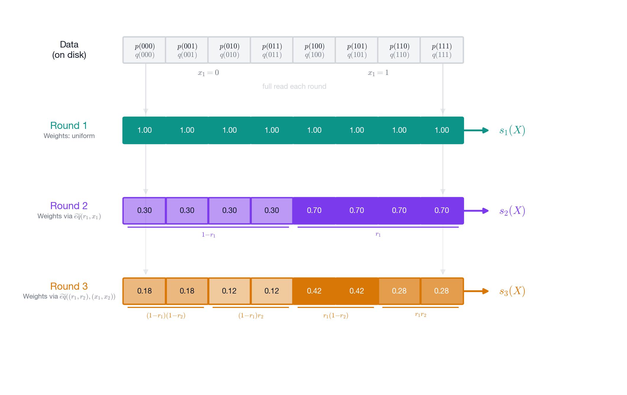
This \( O(\log N) \)-space algorithm allows proving much larger statements than the linear-space approach, limited by disk capacity or regeneration time rather than RAM. In practice, implementations often use a hybrid approach: stream for the first few rounds until the effective problem size shrinks enough to fit in memory, then switch to the faster linear-time algorithm. Even so, the streaming phase can add substantial overhead for large instances (e.g., \( n \approx 30 \)).
New Idea: Round Batching and its Benefits
Both the linear-time and the CMT streaming algorithm share a common structure: they proceed round-by-round . For each round \( i \), the prover computes a univariate polynomial \( s_i(X) \), sends it, waits for the verifier’s challenge \( r_i \), and only then computes the polynomial \( s_{i+1}(X) \) for the next round.
What if we could break this sequential dependency? Instead of computing just one round at a time, could the prover compute, say, rounds 1 and 2 simultaneously? Or any number of consecutive rounds at once?
This is the idea behind round batching , introduced in my work [9] and independently in Baweja et al. [10]. The extended version of my work [9] develops this idea further alongside several complementary optimizations. Round batching can speed up both prover algorithms above, especially in settings relevant to proving program execution.
At first glance, this proposal seems impossible: the prover cannot know the claim for round 2 without knowing the challenge \( r_1 \) from round 1. The key observation is that the prover can compute a response that is oblivious to the future challenges. This is achieved by computing a bivariate polynomial $$ s(X_1, X_2) = \sum_{x’ \in \{0,1\}^{n-2}} p(X_1, X_2, x’) \cdot q(X_1, X_2, x’) $$ that suffices to answer both rounds 1 and 2. Indeed, the first round polynomial \( s_1(X_1) \) is equal to \( s(X_1, 0) + s(X_1, 1) \), and once the prover receives the first challenge \( r_1 \), the second round polynomial \( s_2(X_2) \) is equal to \( s(r_1, X_2) \).
More generally, if we want to compute \( w \) consecutive rounds at once, starting at round \( i \), the prover will need to compute the \( w \)-variate polynomial $$ s(X_1, \dots, X_w) = \sum_{x’ \in \{0,1\}^{n-i-w+1}} p(r_1, \dots, r_{i-1}, X_1, \dots, X_w, x’) \cdot q(r_1, \dots, r_{i-1}, X_1, \dots, X_w, x’). $$ Once the prover has computed this polynomial, the next \( w \) rounds of the protocol reduce to running sum-check on the \( w \)-variate polynomial \( s \) itself: $$ \sum_{x \in \{0,1\}^w} s(x) = c_{i-1}, $$ where \( c_{i-1} \) is the claim at the start of round \( i \), with \( c_0 := c \). This is the same reduction that we saw above for \( i=1 \) and \( w=2 \).
Since \( w \) is often much smaller than \( n \), this inner sum-check is easy; the main cost is computing \( s(X_1, \dots, X_w) \) itself. Because \( s \) is multi-quadratic (degree at most \( 2 \) in each variable), it is determined by its values on the \( \{0,1,2\}^w \) grid. For instance, if \( w = 2 \), one evaluation (say \( s(1,2) \)) is $$ s(1, 2) = \sum_{x’ \in \{0,1\}^{n-i-1}} p(r_1, \dots, r_{i-1}, 1, 2, x’) \cdot q(r_1, \dots, r_{i-1}, 1, 2, x’) $$ $$ \qquad\qquad\quad = \sum_{x’ \in \{0,1\}^{n-i-1}} (2 \cdot p(r_1, \dots, r_{i-1}, 1, 1, x’) - p(r_1, \dots, r_{i-1}, 1, 0, x’)) $$ $$ \qquad\qquad\qquad \cdot (2 \cdot q(r_1, \dots, r_{i-1}, 1, 1, x’) - q(r_1, \dots, r_{i-1}, 1, 0, x’)). $$
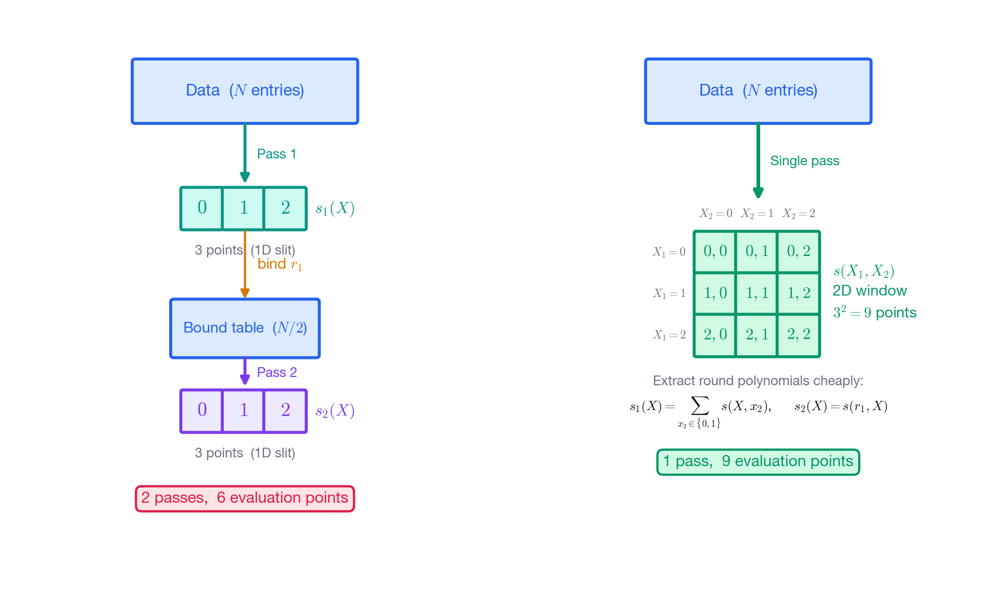
The apparent cost. At first glance, round batching looks slower. Round-by-round sum-check computes \( 3 \) evaluations of a quadratic polynomial per round (or \( d+1 \) evaluations for degree \( d \)). With a batching window \( w \), we compute \( 3^w \) evaluations (or \( (d+1)^w \)) over those \( w \) rounds, instead of \( w \cdot (d+1) \). This gap grows quickly: with \( d = 2 \) and \( w = 3 \), batching computes three times as many evaluations.
Why does round batching help?
The key insight is that the cost of computing evaluations is not equal across all rounds. In particular, there are two settings where round batching leads to a speedup despite the apparent extra work.
Small-field arithmetic at the start. In many proof systems for correct program execution, the underlying data (such as register values or memory contents) are small—typically 64-bit integers—while the proof system operates over a large field (often 128-bit or 256-bit). Arithmetic with 64-bit integers is about 10–50x faster than full field multiplication.
For sum-check involving these small values, the prover enjoys a speedup in the first round, since the original evaluations $$ (p(x), q(x))_{x \in \{0,1\}^n} $$ are small. However, this speedup goes away in later rounds, since the bound evaluations \[ ( p(r_1, \dots, r_{i-1},x), q(r_1, \dots, r_{i-1}, x))_{x \in \{0,1\}^{n-i}} \] are full field elements.
Round batching extends this cheap-multiplication regime to the first \( w>1 \) rounds. Applying batching to the first \( w \) rounds means the prover computes evaluations of $$ s(x_1, \dots, x_w) = \sum_{x’ \in \{0,1\}^{n-w}} p(x_1, \dots, x_w, x’) \cdot q(x_1, \dots, x_w, x’). $$ Since the original evaluations $$(p(x), q(x))_{x \in \{0,1\}^n}$$ are small, the extended evaluations over \( \{0,1,2\}^w \) are also small (they are simple linear combinations). Thus, batching trades expensive field multiplications from rounds \( 2,\dots,w \) for a larger number of much cheaper small multiplications. In practice, \( w \approx 3 \) can yield a \( 2\text{–}3\times \) prover speedup.
Fewer streaming passes. Recall that in the CMT streaming algorithm, the prover needs to make a pass over the original input in every round (or as long as we don’t have space to store the bound evaluations). The cost of each pass is \( O(N) = O(2^n) \), which does not shrink as the protocol progresses.
Round batching reduces the number of passes over the original input: instead of one pass per round within a \( w \)-round window, it needs a single pass at the start of the window. If we batch starting at round \( i \), the added evaluation work scales as \( (d+1)^w \cdot 2^{n-i-w+1} \), while we save about \( (w-1)\cdot 2^n \) work from skipped streaming passes. With an appropriate schedule—small windows early and larger windows later—we can reduce the number of streaming passes asymptotically from \( O(n) \) to \( O(\log n) \). For example, a 30-variable instance would require 30 passes with the baseline streaming algorithm; with round batching at increasing window sizes, this drops to roughly 5 passes, yielding \( 3\text{–}5\times \) speedups in practice.
Conclusion
The sum-check protocol has become the workhorse of modern proof systems, powering a wide range of protocols and sub-protocols such as polynomial commitment schemes [11]. In this post, we have seen the evolution of sum-check proving algorithms: from the classic linear-time prover that trades memory for speed, to the streaming algorithm that sacrifices time for a minimal memory footprint. Both approaches share a common, intuitive pattern: they process rounds sequentially, binding each challenge before moving to the next.
We then saw how round batching breaks this sequential dependency, leading to two practical wins: it keeps arithmetic in fast, small-value operations for longer, and it reduces the number of streaming passes in memory-constrained settings.
One important application of these techniques is in zero-knowledge virtual machines (zkVMs) : systems that can execute a program (compiled to an instruction-set architecture like RISC-V) and produce a cryptographic proof that the execution was correct. Round batching is one of several complementary techniques developed in [9] and integrated into Jolt [3], a state-of-the-art zkVM, where together they yield over \( 10\times \) speedup and \( 17\times \) memory reduction on a key sub-protocol. These improvements make it feasible to prove significantly larger programs on consumer hardware.
As proof systems see broader adoption, every percentage point of prover speedup translates to real cost savings and expanded applicability. It is perhaps surprising that we are still extracting efficiency from sum-check; despite being over three decades old, it continues to admit optimizations tailored to modern constraints.
Citations:
[1] Google. Longfellow ZK: Implementation of the Google Zero-Knowledge library for Identity Protocols. GitHub repository. https://github.com/google/longfellow-zk. See also: Frigo, M., & shelat, a. (2025). The Longfellow Zero-knowledge Scheme (draft-google-cfrg-libzk-01). Internet-Draft, IETF. https://datatracker.ietf.org/doc/draft-google-cfrg-libzk/
[2] EthProofs. EthProofs: Zero-knowledge proofs resources for Ethereum. https://ethproofs.org/
[3] a16z crypto. Jolt: a zkVM for general-purpose computation. GitHub repository. https://github.com/a16z/jolt
[4] Lund, C., Fortnow, L., Karloff, H., & Nisan, N. (1992). Algebraic methods for interactive proof systems. Journal of the ACM, 39(4), 859–868. https://dl.acm.org/doi/10.1145/146585.146605
[5] Schwartz, J. T. (1980). Fast probabilistic algorithms for verification of polynomial identities. Journal of the ACM, 27(4), 701–717.
[6] Vu, V., Setty, S., Blumberg, A. J., & Walfish, M. (2013). A Hybrid Architecture for Verifiable Computation. In Proceedings of the 2013 IEEE Symposium on Security and Privacy (SP), 223–237. IEEE.
[7] Thaler, J. (2013). Time-Optimal Interactive Proofs for Circuit Evaluation. In Advances in Cryptology – CRYPTO 2013 (LNCS 8042, pp. 71–89). Springer.
[8] Cormode, G., Mitzenmacher, M., & Thaler, J. (2012). Practical Verified Computation with Streaming Interactive Proofs. In Proceedings of the 2nd Innovations in Theoretical Computer Science Conference (ITCS 2012), 90–112. ACM.
[9] Dao, Q., DeStefano, Z., Bagad, S., Domb, Y., & Thaler, J. (2026). Speeding Up Sum-Check Proving (Extended Version). Cryptology ePrint Archive, Paper 2026/587. https://eprint.iacr.org/2026/587
[10] Baweja, A., Chiesa, A., Fedele, E., Fenzi, G., Mishra, P., Mopuri, T., & Zitek-Estrada, A. (2025). Time-Space Trade-Offs for Sumcheck. In Theory of Cryptography Conference (TCC 2025).
[11] Arnon, G., Chiesa, A., Fenzi, G., & Yogev, E. (2024). WHIR: Reed–Solomon Proximity Testing with Super-Fast Verification. Cryptology ePrint Archive, Paper 2024/1586. https://eprint.iacr.org/2024/1586
