
Crediting the Right Steps: Stepwise Reward Assignment for RL on Flow Matching Models
Flow matching models like Stable Diffusion 3.5 and FLUX generate an image by iteratively denoising random noise over many small steps. When we want to fine-tune these models with reinforcement learning, say to make them follow text prompts more faithfully or produce more aesthetic outputs, a natural question arises: which steps deserve credit, or blame, for the final result?
The current state of the art, Flow-GRPO , sidesteps this question. Every denoising step gets the same credit, computed from the reward on the final image. If the image is good, every step is reinforced equally. If it is bad, every step is penalized. This is a tempting simplification, but it ignores something important about how diffusion generation actually works. Different steps do fundamentally different things, and treating them identically wastes most of the available learning signal.
This blog post describes our recent work, Stepwise Credit Assignment for GRPO on Flow Matching Models (to appear at CVPR 2026; work done while interning at Adobe Research), which proposes a fix.
TL;DR
- Problem. Flow-GRPO assigns the same advantage to every denoising step in a trajectory, ignoring that early steps determine composition while late steps refine details. A trajectory with bad early decisions that get corrected later is reinforced just as strongly as one with good decisions throughout.
- Stepwise rewards via Tweedie. We score every denoising step by applying the reward model to a few-step Tweedie estimate \(\hat{x}_{0}(t) = \mathbb{E}[x_{0} \mid x_{t}]\) of the clean image from the noisy state. This is essentially free since \(\hat{x}_{0}(t)\) reuses the predicted noise that the flow model already computes at every step.
- Stepwise gains, not raw rewards. We optimize the per-step gain \(g_{t} = r_{t-1} - r_{t}\). The gains telescope to the total reward improvement, so we get fine-grained credit assignment without changing the global objective.
- Improved SDE. Flow-GRPO’s SDE matches the flow ODE marginals correctly, but its particular parameterization produces visibly noisy final samples that degrade the reward signal. We replace it with a DDIM-inspired alternative that keeps intermediate samples clean.
- Results. Stepwise-Flow-GRPO has better sample efficiency than Flow-GRPO , in both training iterations and wall-clock time, across three reward models (PickScore, ImageReward, UnifiedReward) on two prompt sets. The improved SDE accelerates both methods, and combining the two changes gives the best results overall. Stepwise-Flow-GRPO also trains stably where Flow-GRPO diverges, including on the 7B UnifiedReward VLM and on OCR text rendering.
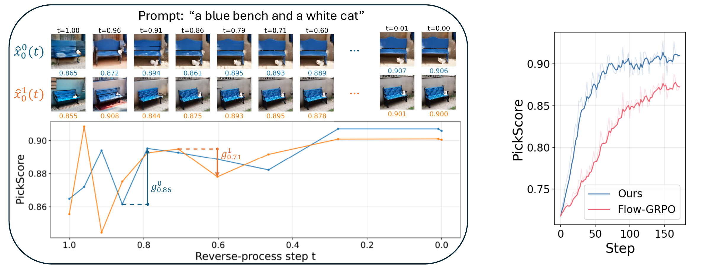
Figure 1. Two denoising trajectories from the same prompt reach roughly the same final reward (about 0.90), but they take very different paths. Trajectory 0 dips at \(t=0.86\) before recovering; trajectory 1 drops sharply at \(t=0.71\). Flow-GRPO’s uniform credit assignment cannot tell them apart. Stepwise-Flow-GRPO can, and uses that distinction to learn faster.
Background
I will set up just enough background to make the rest of the post self-contained. Readers familiar with flow matching and GRPO can safely skip ahead.
Flow Matching
Flow matching is a recent reframing of diffusion modeling that has become the dominant approach in state-of-the-art image generators, including Stable Diffusion 3 / 3.5 and the FLUX family. The version we use, rectified flow , is built around a simple linear interpolant. Given a clean data sample \(x_{0} \sim p_{\text{data}}\) and Gaussian noise \(x_{1} \sim \mathcal{N}(0, I)\), define
\[ x_{t} = (1-t) x_{0} + t x_{1}, \qquad t \in [0, 1] \]
so that \(x_{0}\) is a clean image, \(x_{1}\) is pure noise, and \(x_{t}\) smoothly interpolates between them. The model \(v_{\theta}(x_{t}, t, c)\) is trained to predict the velocity \(\dot{x}_{t} = x_{1} - x_{0}\) of this interpolant at time \(t\), conditioned on a prompt \(c\):
\[ \mathcal{L}(\theta) = \mathbb{E}_{t, x_{0}, x_{1}} \left[ \lVert (x_{1} - x_{0}) - v_{\theta}(x_{t}, t, c) \rVert^{2} \right] \]
To generate an image, we start from pure noise \(x_{1} \sim \mathcal{N}(0, I)\) at \(t=1\) and integrate the learned ODE \(dx_{t} = v_{\theta}(x_{t}, t, c) dt\) backward to \(t=0\). In practice we discretize this integration into \(T\) steps (the denoising steps I will refer to throughout).
Converting the ODE to an SDE for RL
The deterministic ODE works fine for inference, but it is not suitable for reinforcement learning. RL needs to explore: from the same prompt and same initial noise, we need the model to produce different trajectories that we can reward differently and compare against each other. A deterministic process produces one trajectory per starting point, so there is nothing to compare.
Following Flow-GRPO , we replace the deterministic ODE with a stochastic differential equation (SDE) that injects a small amount of noise at each step. Both the ODE and the SDE are run starting from the same noise distribution \(x_{1} \sim \mathcal{N}(0, I)\), and the SDE is carefully constructed so that, at every time \(t\), the distribution of \(x_{t}\) is the same under both processes. This marginal-preserving property keeps RL training aligned with the deterministic ODE we use at inference. After discretization, each denoising step becomes a draw from a Gaussian:
\[ \pi_{\theta}(x_{t-\Delta t} \mid x_{t}, c) = \mathcal{N}(x_{t-\Delta t};\ \mu_{t},\ \sigma_{t}^{2} \Delta t \cdot I) \]
where the mean \(\mu_{t}\) is determined by the velocity prediction \(v_{\theta}\) and \(\sigma_{t}\) is a noise schedule we choose. Now we have a stochastic policy \(\pi_{\theta}\) that we can optimize: each rollout of the sampler produces a different trajectory \((x_{T}, x_{T-1}, \ldots, x_{0})\) ending in a different final image.
GRPO
GRPO is the policy optimization algorithm introduced in DeepSeekMath (Shao et al., 2024) and later popularized by DeepSeek-R1 . It is appealingly simple, and crucially it avoids needing a learned critic network (more on that below).
For each prompt \(c\), we sample \(N\) trajectories from the current policy and compute each one’s reward \(r^{i}\) for \(i = 1, \ldots, N\). We then standardize the rewards within this group of \(N\):
\[ A^{i} = \frac{r^{i} - \mu}{\sigma}, \qquad \mu = \frac{1}{N} \sum_{j=1}^{N} r^{j}, \qquad \sigma = \sqrt{\frac{1}{N} \sum_{j=1}^{N} (r^{j} - \mu)^{2}} \]
The standardized reward \(A^{i}\), called the group-relative advantage , measures how much better trajectory \(i\) performed than the average trajectory in its group, in units of standard deviations.
We then update the policy by gradient ascent on a clipped surrogate objective. For each step \(t\) of trajectory \(i\), we compute the propensity ratio
\[ \rho_{t}^{i}(\theta) = \frac{\pi_{\theta}(x_{t}^{i} \mid x_{t+1}^{i}, c)}{\pi_{\text{old}}(x_{t}^{i} \mid x_{t+1}^{i}, c)} \]
which is how much more (or less) likely the current policy \(\pi_{\theta}\) is to take the action that the sampling policy \(\pi_{\text{old}}\) actually took. The objective is
\[ J(\theta) = \frac{1}{NT} \sum_{i=1}^{N} \sum_{t=0}^{T-1} \left[ \min\left(\rho_{t}^{i} A^{i},\ \mathrm{clip}(\rho_{t}^{i}, 1-\varepsilon, 1+\varepsilon)\ A^{i}\right) - \beta\ \mathrm{KL}(\pi_{\theta} \mid\mid \pi_{\text{ref}}) \right] \]
The two stabilization mechanisms are:
- Ratio clipping. If the current policy diverges too much from the sampling policy \((|\rho - 1| > \varepsilon)\), the clipped term pins the gradient and prevents destructively large updates.
- KL regularization. The KL penalty pulls the policy toward a fixed reference policy \(\pi_{\text{ref}}\), typically the model before any RL fine-tuning. This anchors the model so it does not lose its general capabilities while adapting to the reward.
Notably, GRPO uses no learned critic or value function. The group mean \(\mu\) plays the role of a baseline, computed from a small batch of rollouts rather than fit by a separate network. This makes GRPO simple to implement, but it means each trajectory gets a single scalar advantage \(A^{i}\), with no fine-grained information about which steps within the trajectory contributed to the reward.
Flow-GRPO
Flow-GRPO applies GRPO to flow matching by sampling \(N\) trajectories from the SDE policy for each prompt \(c\), computing the reward on each final image \(r^{i} = R(x_{0}^{i}, c)\), and propagating the corresponding advantage scalar \(A^{i}\) to every denoising step in the trajectory. That is, every step \(t = 0, 1, \ldots, T-1\) in trajectory \(i\) sees the same \(A^{i}\). This is the design choice we challenge.
Why Uniform Credit Assignment is Wasteful
Flow-GRPO leaves performance on the table, for two related reasons.
Problem 1: Diffusion has a temporal hierarchy. Different denoising steps do qualitatively different work. Early steps (when \(t\) is close to 1 and most of the signal is still noise) establish coarse structure: object layout, composition, color blocking. Late steps (when \(t\) is close to 0 and the image is nearly clean) refine high-frequency details: textures, sharp edges, fine geometry. This coarse-to-fine progression is a well-known property of diffusion generation, and the paper walks through a quick frequency-domain derivation. Uniform credit assignment ignores this structure, treating all denoising steps equally regardless of which role they play.
Problem 2: The final image hides what happened along the way. Only rewarding the final image may unintentionally reinforce early steps that made mistakes which got corrected later in the trajectory. Figure 1 above shows some of this non-monotonic variability across trajectories.
Stepwise-Flow-GRPO
The plan is straightforward. Instead of one reward per trajectory, compute a reward at every step, and credit each step based on its improvement (or gain ) over the previous step. Two challenges to address: (1) reward models are trained on clean images, so they do not give meaningful scores on the noisy intermediate states \(x_{t}\) that come up mid-trajectory; and (2) we need to be careful that introducing per-step rewards does not push the model away from the final-image objective we actually care about.
Estimating Intermediate Rewards via Tweedie’s Formula
We address challenge (1) using Tweedie’s formula, which gives us a posterior-mean estimate of the clean image from the noisy state:
\[ \hat{x}_{0}(t) := \mathbb{E}[x_{0} \mid x_{t}] = x_{t} - t \hat{x}_{1} \]
where \(\hat{x}_{1}\) is the predicted noise, already computed at every step during sampling. We score the Tweedie estimate instead of \(x_{t}\) itself: \(r_{t}^{i} = R(\hat{x}_{0}^{i}(t), c)\). The one-step Tweedie estimate is essentially free since it reuses computation we are already doing.
The one-step estimate is not always sharp, though, especially when \(t\) is far from 0 and \(x_{t}\) is still mostly noise. We get a sharper estimate by taking \(x_{t}\) and running it forward through the flow ODE for a few extra steps toward \(t = 0\), producing a cleaner image to feed to the reward model. The number of extra ODE substeps \(T’\) trades off estimate quality against compute. We use \(T’ = 5\), which the paper’s ablations show gives a strong reward signal without much overhead.
Because the denoising and rewarding from each \(x_{t}^{i}\) is independent, all \(T\) reward estimates for a trajectory can be computed in parallel, which keeps the wall-clock overhead manageable.
Gains, Not Raw Rewards
The more natural GRPO extension would be to compute per-step advantages directly from the intermediate rewards \(r_{t}^{i}\), standardizing them within the group just as Flow-GRPO standardizes the final reward. But this is the wrong objective: it tells the model to make Tweedie estimates score well at every point along the trajectory, even very early on. A Tweedie estimate from a noisy mid-trajectory state is a blurry guess at the final image, not the final image itself. Pushing it to score highly distorts the denoising dynamics and pulls the model away from producing high-quality final outputs, which is what we actually care about.
The fix is to credit each step by its gain , the improvement it produces over the previous step:
\[ g_{t}^{i} := r_{t-1}^{i} - r_{t}^{i} \]
The crucial property is that gains telescope:
\[ \sum_{t=1}^{T} g_{t}^{i} = r_{0}^{i} - r_{T}^{i} \]
So summing per-step gains across the trajectory recovers the total improvement from initial noise \(x_{T}\) to final image \(x_{0}\). And because all \(N\) trajectories in a group share the same initial noise \(x_{T}\), the term \(r_{T}^{i}\) is identical across the group. After group-relative normalization (subtracting the mean over the group), this shared constant drops out, leaving us optimizing exactly the group-relative final reward, the same thing Flow-GRPO optimizes. The difference is that we now have per-step credit along the way, without changing the global objective.
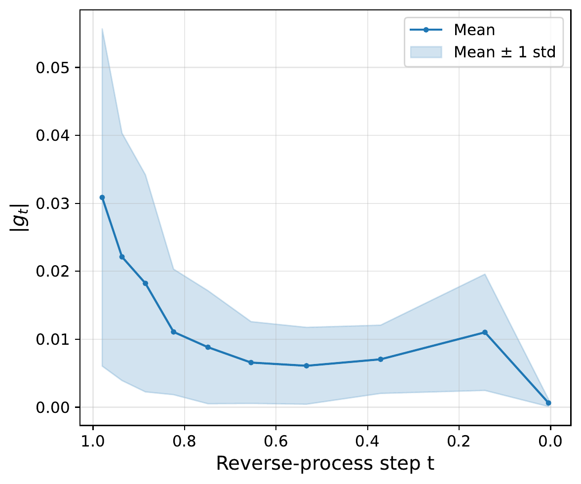
Figure 2. Mean absolute gain per denoising step, measured on 256 GenEval prompts using PickScore. Gains are largest near \(t = 1\) and shrink as denoising progresses. Most reward improvement comes from early compositional decisions, with later steps making smaller refinements. This matches the frequency-hierarchy story from earlier and gives the optimization a natural prior toward the steps that matter most.
Joint Normalization
We compute group-relative advantages, but we normalize jointly across all steps and trajectories rather than per-step:
\[ \tilde{A}_{t}^{i} = \frac{g_{t}^{i} - \mu_{\text{global}}}{\sigma_{\text{global}}} \]
where, unlike the background GRPO definition that averaged only over the \(N\) trajectories, \(\mu_{\text{global}}\) and \(\sigma_{\text{global}}\) are computed over the \(NT\) pairs \((i, t)\), i.e., across both trajectories and timesteps:
\[ \mu_{\text{global}} = \frac{1}{NT} \sum_{i=1}^{N} \sum_{t=1}^{T} g_{t}^{i}, \qquad \sigma_{\text{global}} = \sqrt{\frac{1}{NT} \sum_{i=1}^{N} \sum_{t=1}^{T} (g_{t}^{i} - \mu_{\text{global}})^{2}} \]
Why joint rather than per-step? Per-step normalization would inflate noise in late steps where reward changes are small, washing out the signal where it is meaningful. Joint normalization preserves the natural temporal structure: early gains are bigger (Figure 2), so they get bigger advantages. An ablation in the paper confirms that joint normalization converges substantially faster.
Pseudocode
The algorithm is essentially Flow-GRPO with the gain computation and joint normalization swapped in:
# All N trajectories in a group share the same initial noise x_T
x_T ~ N(0, I)
for i in range(N):
    x[i, T] = x_T
    for t in range(T-1, -1, -1):
        x[i, t] ~ pi_theta( . | x[i, t+1], c)               # SDE step
    for t in range(T + 1):
        x_hat_0[i, t] = denoise(x[i, t], substeps=T_prime)  # Tweedie estimate
        r[i, t]       = R(x_hat_0[i, t], c)                 # reward at step t

# Stepwise gains for t = 1, ..., T
for i in range(N):
    for t in range(1, T + 1):
        g[i, t] = r[i, t-1] - r[i, t]

# Joint normalization across all i, t
A_tilde = (g - mean(g)) / std(g)

# Standard GRPO update with A_tilde[i, t] instead of trajectory advantage A^i
optimize(theta, A_tilde, propensity_ratio, KL_penalty)
That is the entire method. The change from Flow-GRPO is small in code and large in effect.
As a side note, the gain formulation also has theoretical grounding in adaptive submodular optimization. Kveton et al. (2025) showed that KL-regularized policy gradients on per-step gains learn near-optimal policies under a monotone-submodular assumption on the reward, and the on-policy version of our objective reduces algebraically to theirs. We do not verify submodularity for the reward functions we use, but the diminishing gains in Figure 2 are at least consistent with that kind of structure. See the paper for details.
An Improved SDE: A Complementary Fix
There is a separate issue with Flow-GRPO that we noticed while developing stepwise credit assignment. The final images produced by Flow-GRPO’s SDE are visibly noisier than those produced by the deterministic flow ODE, especially when sampling with fewer denoising steps. This is somewhat surprising at first glance, because the Flow-GRPO SDE provably matches the marginals of the flow ODE. The catch is that marginal matching is a statement about the distribution of \(x_{t}\) across many rollouts. It does not say anything about how clean any individual rollout looks. Flow-GRPO’s particular SDE has enough noise injection at each step that single rollouts come out visibly degraded, even though the distribution across many rollouts matches the flow ODE. Since reward models are evaluated on individual images and were trained on clean ones, this degrades the reward signal regardless of the credit assignment scheme. So we replaced Flow-GRPO’s SDE with a DDIM -inspired alternative.
The new update rule interpolates between deterministic and stochastic sampling:
\[ x_{t-\Delta t} = (1 - (t-\Delta t)) \hat{x}_{0}(t) + \sqrt{(t-\Delta t)^{2} - \sigma_{t}^{2}} \hat{x}_{1} + \sigma_{t} \epsilon \]
The key design property is that setting \(\sigma_{t} = 0\) zeroes out the noise term and recovers the deterministic flow ODE exactly, so we can dial in the amount of stochasticity we want for RL training.
There is a tradeoff. Marginal matching to the flow ODE (the property that Flow-GRPO’s SDE achieves exactly) only holds for our SDE in the Taylor limit of small \(\sigma_{t}\). For the small \(\sigma_{t}\) we use in practice, the approximation is tight enough that the SDE remains a useful training surrogate for the ODE sampler we use at inference. The paper gives the formal Taylor-limit argument and variance calculation.
The noise schedule \(\sigma_{t}\) itself is a free choice. We propose a particular schedule chosen to maximize the useful training signal across timesteps; see the paper for the form and the design rationale.
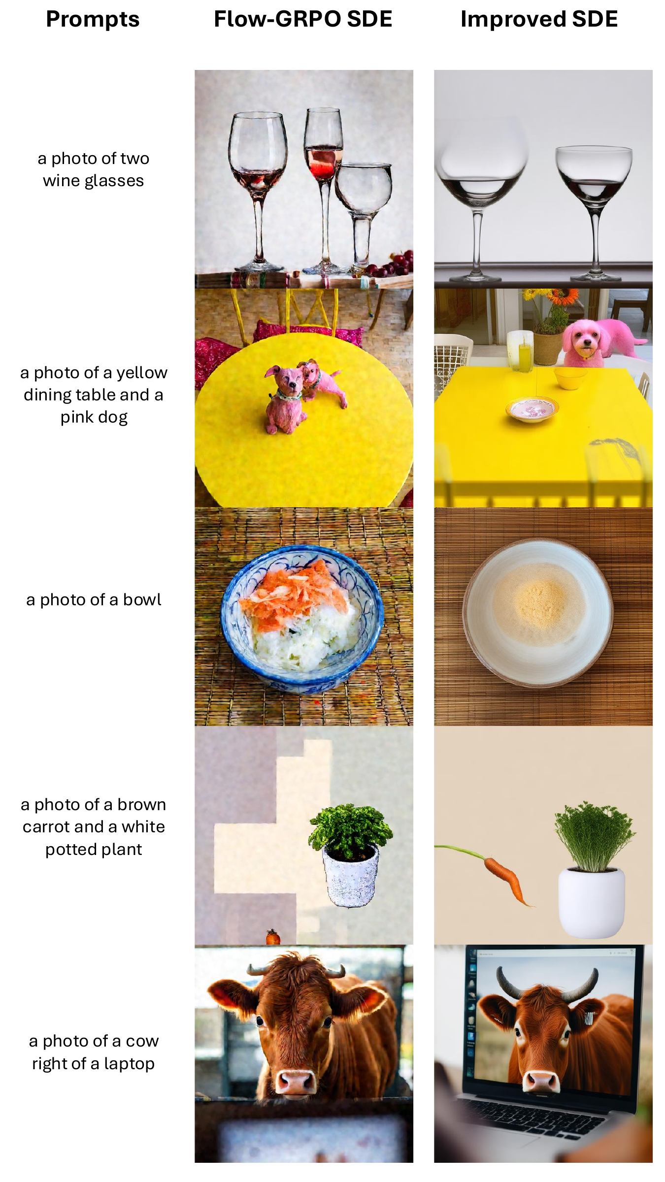
Figure 3. Final images sampled with each SDE. Flow-GRPO’s SDE produces visibly noisy results (middle column); our DDIM-inspired SDE produces clean images (right column) while still injecting enough stochasticity for policy gradients.
Experiments
We trained Stable Diffusion 3.5-Medium with both methods in four configurations: three reward models on GenEval prompts ( PickScore , a lightweight CNN trained on human preferences; ImageReward , a larger transformer also trained on human preferences; and UnifiedReward-7B , a 7B vision-language model that scores both prompt alignment and visual quality), plus PickScore on its own prompt set.
Sample efficiency
Figure 4 shows reward against training step for each reward-prompt combination. The headline finding is that Stepwise-Flow-GRPO reaches any given reward level in substantially fewer training steps than Flow-GRPO; the gap is largest early in training. This is the main result of the paper. The picture is the same in wall-clock time (the paper has the plot), though the gap there is less dramatic since each Stepwise-Flow-GRPO iteration costs more (it runs the reward model on \(T\) Tweedie estimates per trajectory instead of just one).
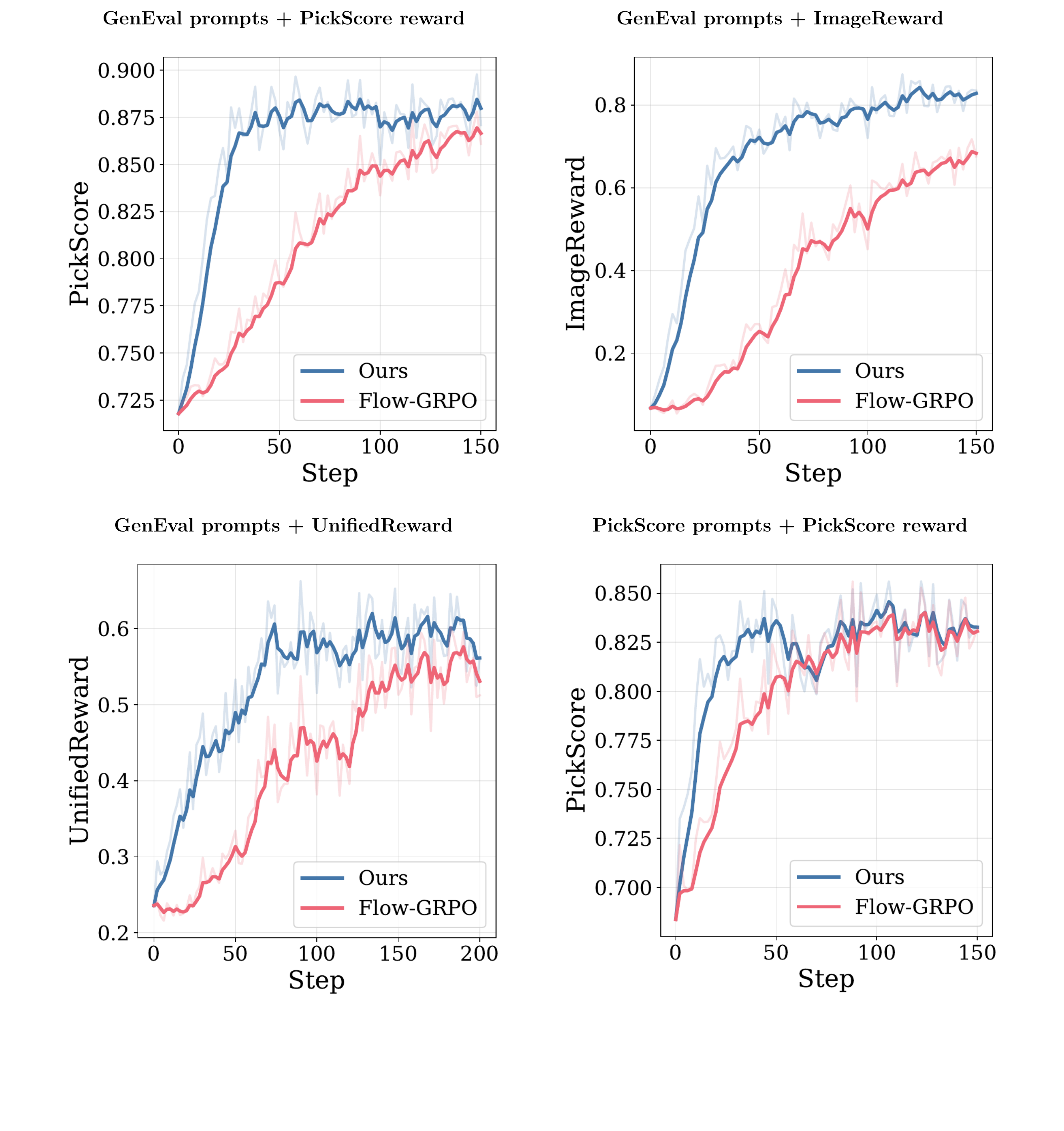
Figure 4. Reward versus training step for Stepwise-Flow-GRPO (blue) and Flow-GRPO (red). The top row and bottom-left panel use GenEval prompts with PickScore, ImageReward, and UnifiedReward respectively; the bottom-right panel uses PickScore prompts with PickScore as the reward.
Improved SDE composes with stepwise credit assignment
Swapping the SDE is an independent intervention, so we also reran Flow-GRPO and Stepwise-Flow-GRPO using the DDIM-inspired SDE.
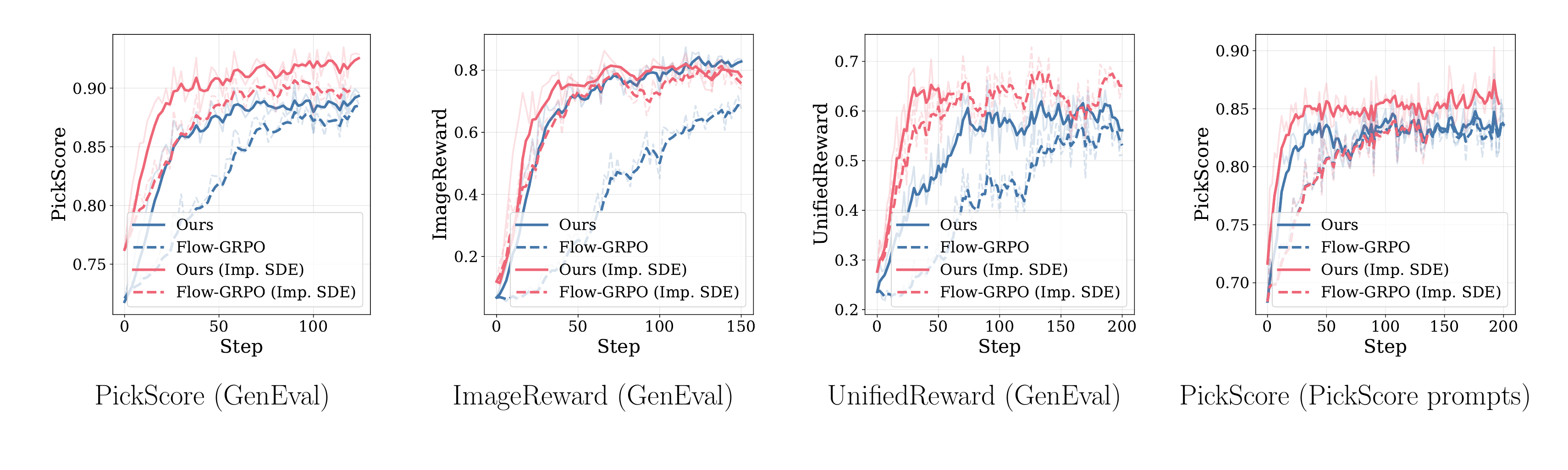
Figure 5. Reward versus training step when both methods use the DDIM-inspired SDE. Stepwise-Flow-GRPO retains its sample-efficiency advantage across PickScore, ImageReward, UnifiedReward, and PickScore prompts, showing that the credit-assignment fix and the sampling fix are complementary.
Stability
There are a few cases where the stepwise method is not just faster but qualitatively more reliable:
UnifiedReward (7B VLM). Under extended training, Flow-GRPO with the standard SDE consistently diverged when trained against UnifiedReward. Stepwise-Flow-GRPO trained stably across runs. Per-step credit appears to keep the policy under control even when the reward gradient is noisy, which it tends to be with large VLM-based rewards.
OCR text rendering. Trained against a combined OCR + PickScore reward, Flow-GRPO diverges after about 500 steps. Stepwise-Flow-GRPO keeps improving past 2000 steps. Text rendering is intuitively a stress test for credit assignment because letter shapes and spacing have to be locked in early and sharpened late.
Final quality on GenEval
To check that the sample-efficiency gains carry over to final image quality, we ran extended training (400 GPU hours) on GenEval rewards and evaluated on the full GenEval benchmark. Stepwise-Flow-GRPO reaches 0.87 overall , with the biggest gains on the categories that demand precise compositional decisions: counting, spatial positioning, and attribute binding.
| Model | Overall | Counting | Position | Attr. Binding |
|---|---|---|---|---|
| SD3.5-M (base) | 0.63 | 0.50 | 0.24 | 0.52 |
| Flow-GRPO (400 GPU hrs) | 0.72 | – | – | – |
| GPT-4o | 0.84 | 0.85 | 0.75 | 0.61 |
| Stepwise-Flow-GRPO (400 GPU hrs) | 0.87 | 0.89 | 0.73 | 0.80 |
Qualitatively, Flow-GRPO fails on the kinds of compositional prompts that demand getting object layout right early: prompts like “a donut below a cat” or “a bus above a boat” frequently come out merged or physically implausible (e.g. a bus floating in the sky). Stepwise-Flow-GRPO is far more consistent on these prompts.
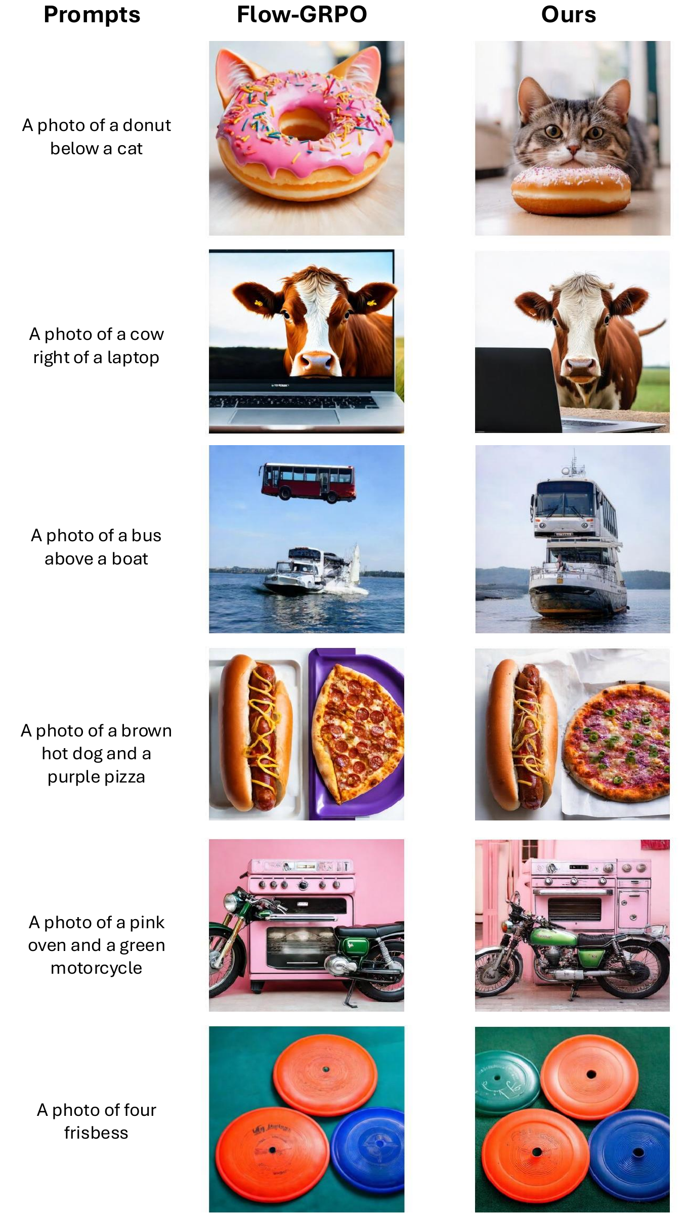
Figure 6. Side-by-side qualitative comparison on GenEval prompts (Flow-GRPO left, Stepwise-Flow-GRPO right). Flow-GRPO merges objects in rows 1 and 5, and produces a bus floating above the water in row 3. Stepwise-Flow-GRPO produces cleaner compositions with better spatial reasoning, attribute binding, and counting.
Discussion
Stepwise-Flow-GRPO replaces Flow-GRPO’s single trajectory-level advantage with per-step gains computed from Tweedie estimates of the clean image, which is most of where the sample-efficiency win comes from. The DDIM-inspired SDE is a separate, simpler fix that helps both methods.
We also tried a few design variations of stepwise credit assignment that we expected might help: an EMA baseline to reduce per-step variance, GAE over the gain sequence, and an ODE-based progressive distillation variant. None outperformed the straightforward gain formulation.
A few natural follow-ups from this work are using per-prompt gain variance as a candidate signal for curriculum learning, and using the gains at inference time as well to detect and re-do bad intermediate denoising steps. See the paper for ablations on the number of denoising substeps, normalization strategies, and a comparison to concurrent work that addresses the same problem from different angles.
