In this blog, we explain the recent progress on an important class of stochastic sequential decision problems, called restless bandits , based on our paper Unichain and aperiodicity are sufficient for asymptotic optimality of average-reward restless bandits . We will also briefly mention the generalization to multiple-actions, multiple-constraints, and heterogeneous arms in the follow-up paper Projection-based Lyapunov method for fully heterogeneous weakly-coupled MDPs .

The rest of the blog is organized as follows. Section 1 motivates the problem with a simple example; Section 2 gives a formal model; Section 3 outlines the construction of our policy; Section 4 states the main optimality result and sketches the proof idea; and Section 5 discusses extensions.

Motivating Problem: Flappy Bird for Octopus

Flappy Bird is an arcade-style mobile game that once went viral around 2014. In this game, a bird flies through a forest of pipes, and the player controls the vertical movements of the bird to avoid the pipes; the goal is to pass as many pipes as possible before hitting a pipe. Despite appearing simple, Flappy Bird is a very hard game for humans. Even for dexterous players, it requires a lot of attention and effort; for beginners, it is all about luck.

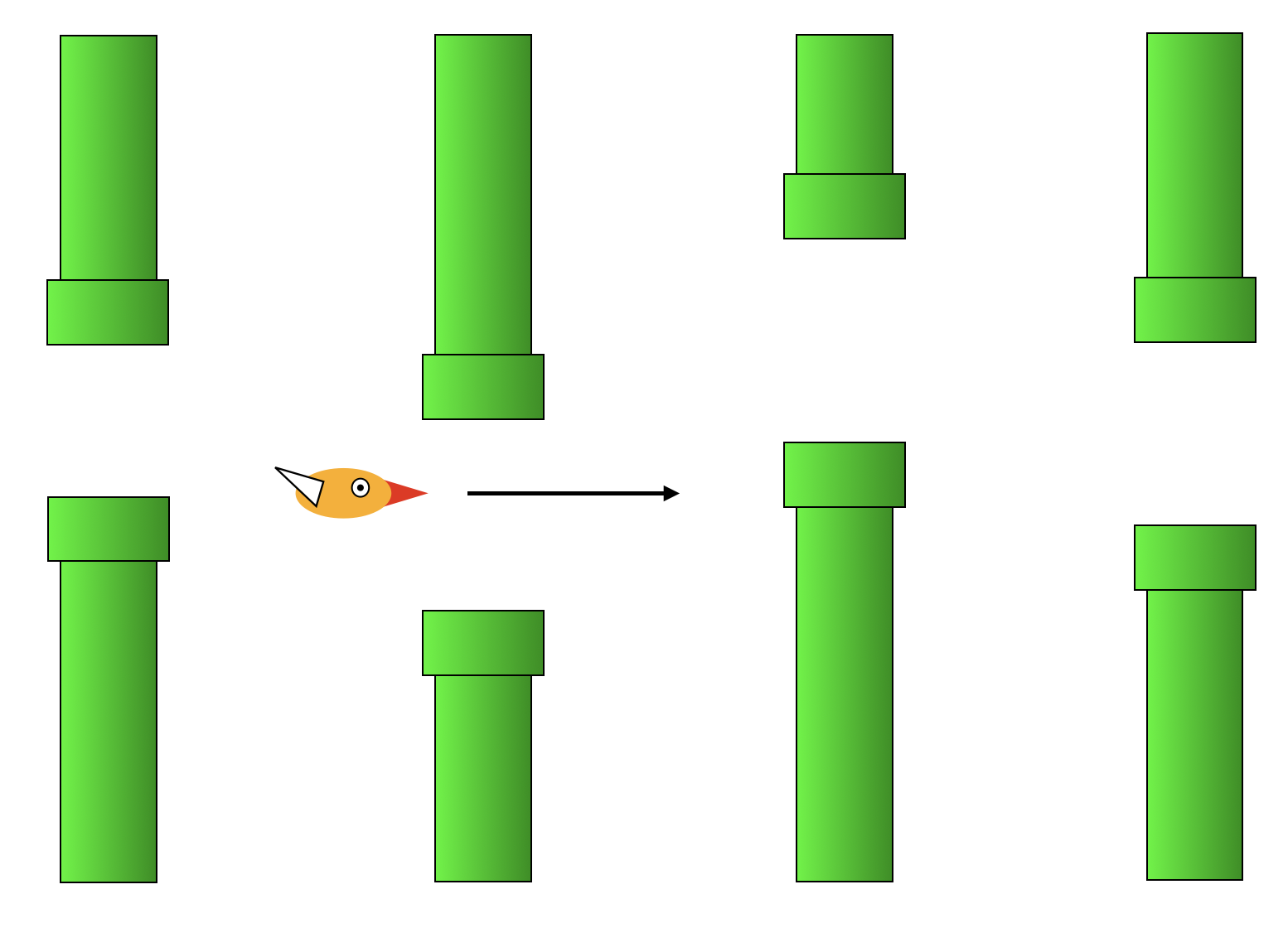
A smart octopus named Sakiko tries to simultaneously play multiple sessions of this game to demonstrate its superiority to humans. Here is what Sakiko can do:

• Sakiko has \(N\) arms and can play Flappy Bird on \(N\) devices simultaneously.
• At any moment, Sakiko can choose to focus on any \(\alpha N\) arms for some fixed \(0 < \alpha < 1\) such that \(\alpha N\) is an integer.
  • The focused arms operate at a high precision and never make mistakes.
  • The rest of the arms operate at a lower precision. These arms could make mistakes with probability \(p\) for some fixed \(0 < p < 1\) when the vertical spaces between pipes are narrow; when the spaces are wide, these arms do not make mistakes.

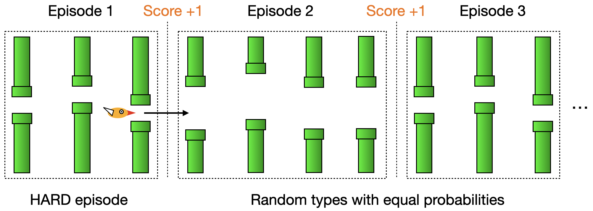
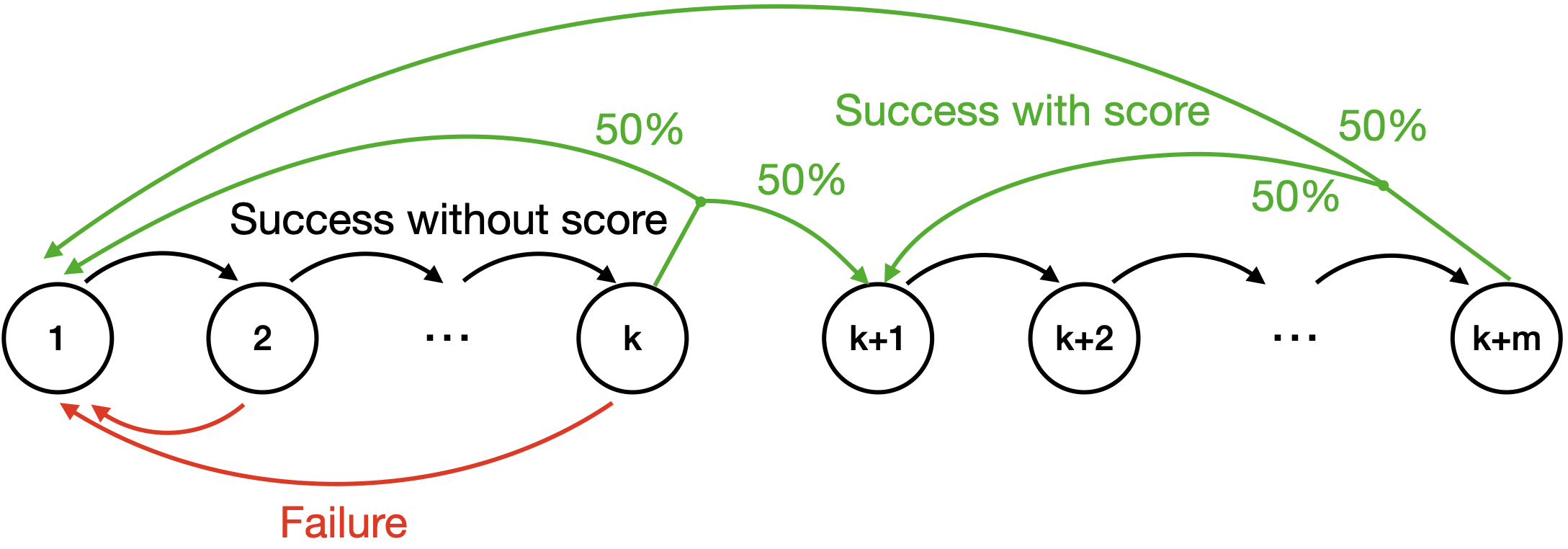
Now consider a version of Flappy Bird that consists of infinitely many episodes , each with multiple pipes. When the bird reaches the end of an episode, it enters a new episode and receives a unit of score; when the bird hits a pipe, the game restarts from the initial episode, with no score generated. There are two types of episodes, HARD (with narrow spaces) or EASY (with wide spaces), and they can have different numbers of pipes. The first episode after restart is always HARD, whereas each subsequent episode’s type is sampled to be HARD or EASY with equal probability each time the bird enters it — so for example, an EASY episode can be followed by a HARD one, while a failure always resets the bird to a HARD episode. The setting is illustrated in Figure 3 below.

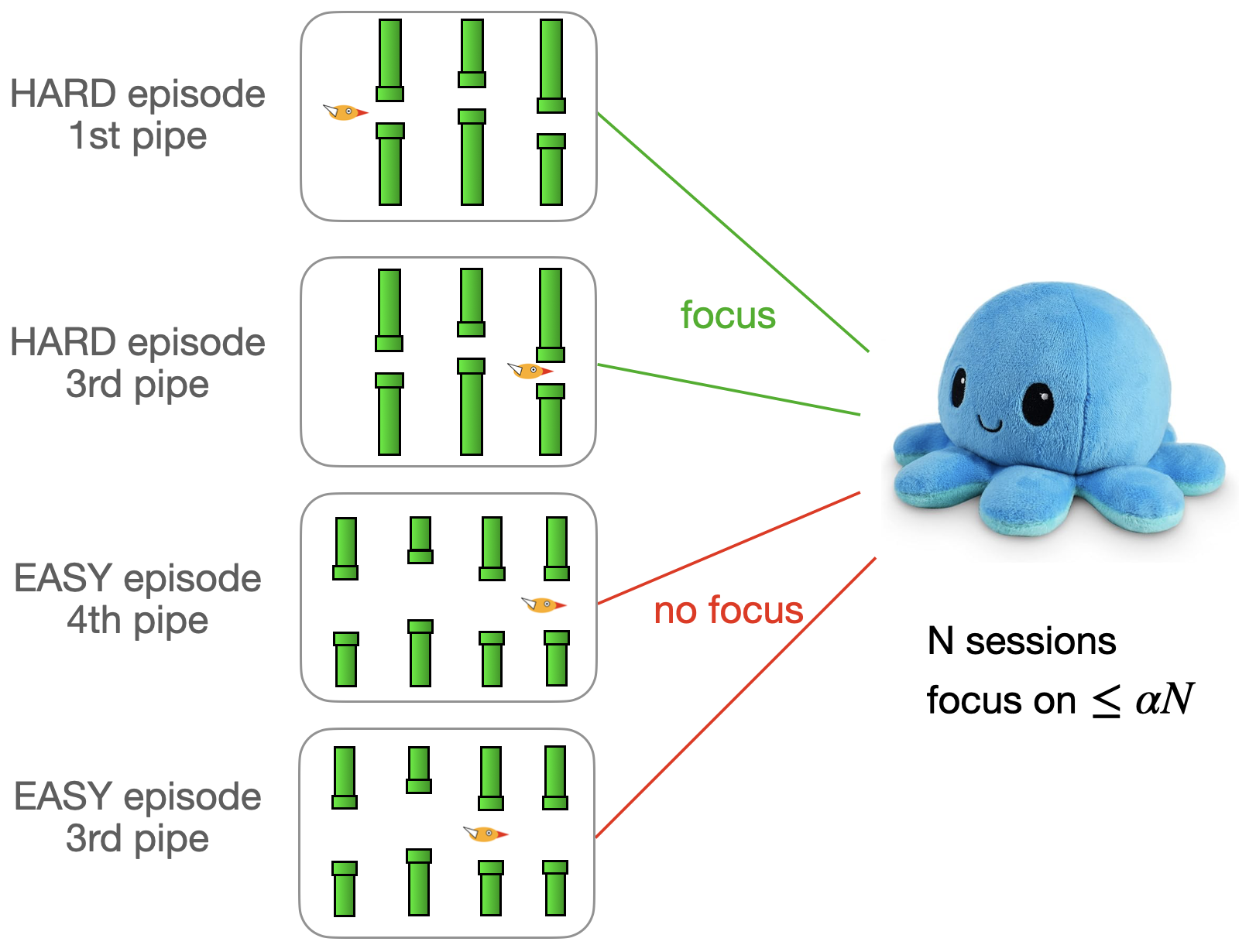
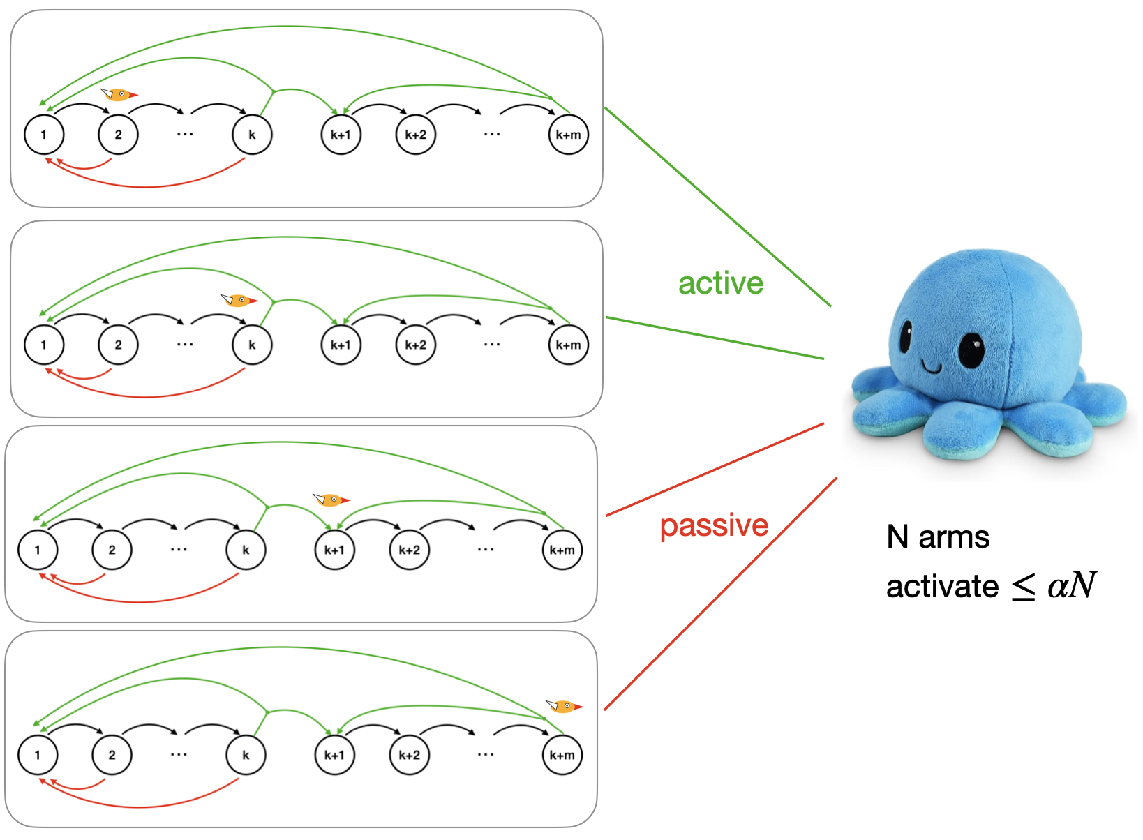
As illustrated in Figure 4 , Sakiko’s goal is to play \(N\) sessions of Flappy Bird simultaneously and maximize the long-run average score per unit of time by choosing the right subset of sessions to focus on. We call this problem the Flappy-Bird-Octopus problem. The rules of the Flappy-Bird-Octopus problem are concretely summarized as follows:

• The problem operates in discrete time, with time steps indexed by \(t=0,1,2,\dots\)
• In each of the \(N\) sessions and at each time step, the bird attempts to pass one pipe, and Sakiko needs to decide whether to focus on this session.
  • If Sakiko focuses on this session, the bird will pass the pipe with probability \(1\).
  • If Sakiko does not focus on this session,
    • If this session is EASY, the bird will still pass the pipe with probability \(1\).
    • If this session is HARD, the bird will still pass the pipe with probability \(1-p\) and hit the pipe with probability \(p\).
  • After passing a pipe,
    • the bird moves on to the next pipe within this episode, or
    • if this is the last pipe in this episode, the bird moves to the first pipe in a new episode and receives \(1\) unit of score. The type of the new episode is HARD or EASY with \(50\%\) probability.
  • After hitting a pipe,
    • the bird restarts from the first pipe in a HARD episode with no score.

Naively, Sakiko could focus on a fixed set of \(\alpha N\) sessions throughout the game, but a smarter strategy is to allocate her focus adaptively — only focusing on the sessions that actually need it, i.e., those currently in a HARD episode. But this still leaves a non-trivial decision: when more than \(\alpha N\) sessions are in HARD episodes, which ones should she focus on? Depending on each session’s progress within its current episode, different rules can lead to dramatically different outcomes.

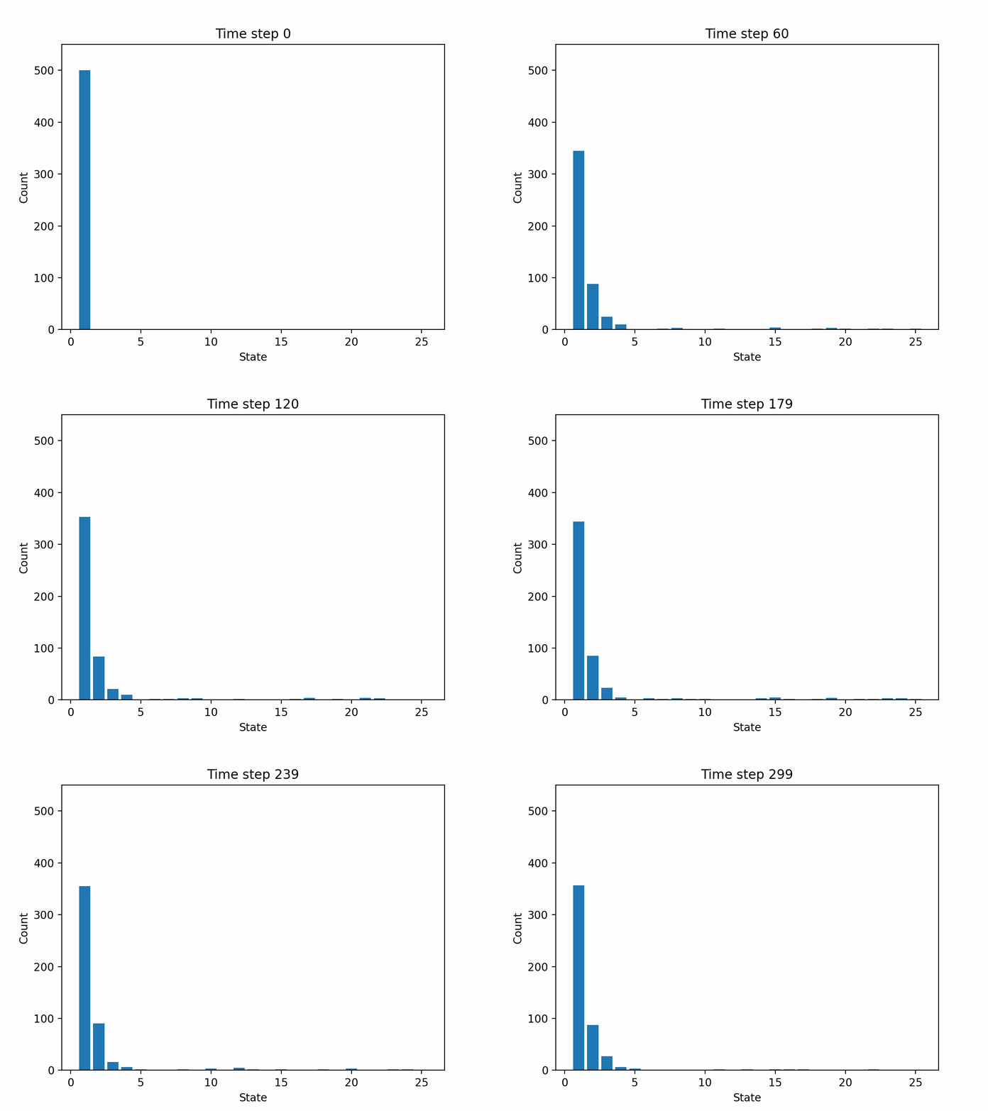
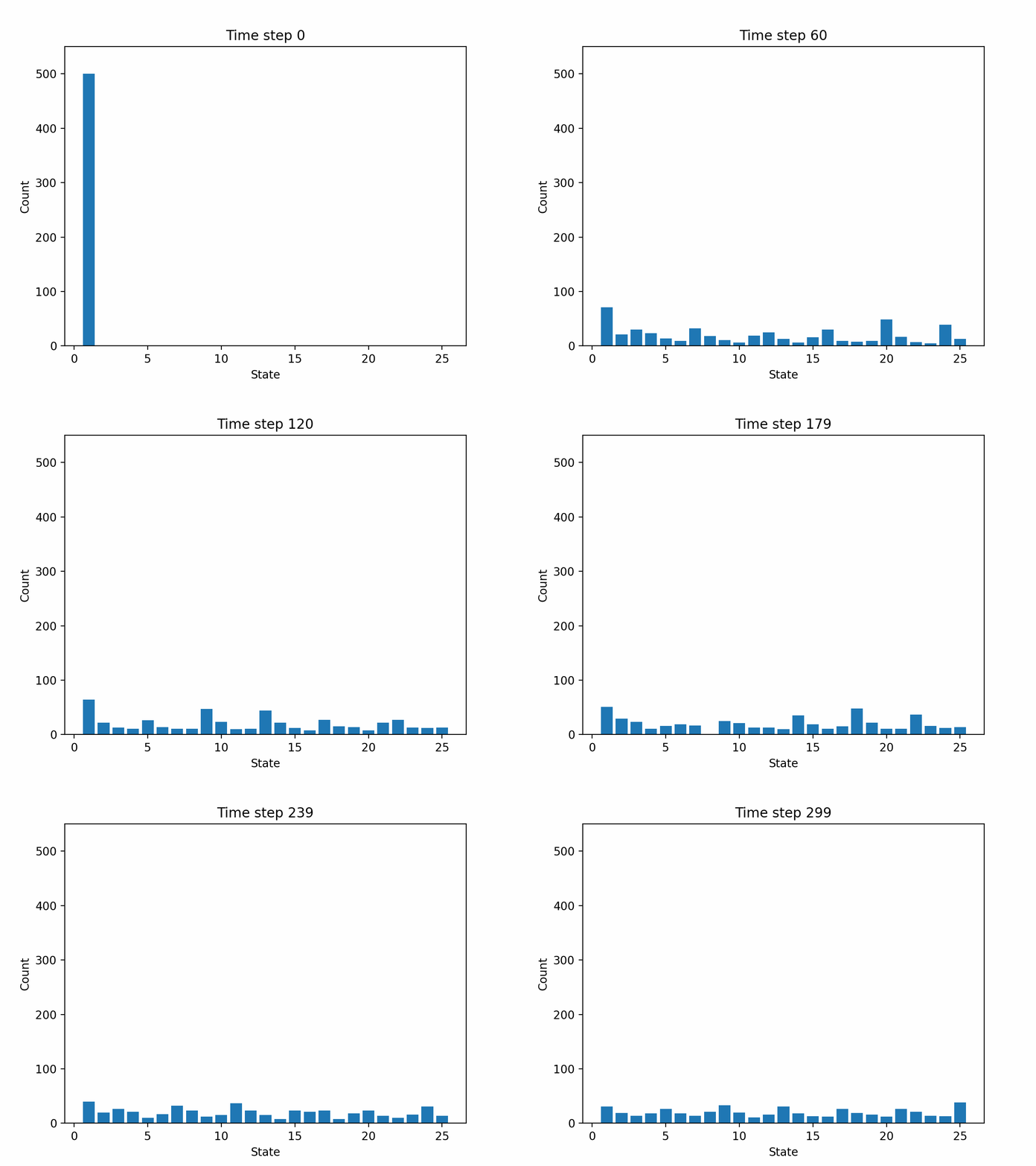
Figure 5 and Figure 6 below illustrate two such rules through simulations with \(N = 500\) sessions. Here, each HARD episode has length \(4\), each EASY episode has length \(21\), and \(\alpha = 4/25\), so Sakiko has just enough budget to focus on all HARD-episode sessions when sessions are spread uniformly across the \(25\) possible (episode type, pipe) pairs. Both figures are histograms whose horizontal axis indexes these \(25\) pairs: the first \(4\) bins correspond to pipes in a HARD episode, and the remaining \(21\) bins to pipes in an EASY episode. The height of each bar counts how many of the \(N\) sessions currently sit at that pair, and the animation shows how this distribution evolves over time.

In Figure 5, when more than \(\alpha N\) sessions are in HARD episodes, Sakiko picks \(\alpha N\) of them uniformly at random to focus on. The outcome is poor: most birds remain piled up at the very first pipes, repeatedly hitting them and restarting from scratch — almost no session ever reaches an EASY episode. In Figure 6, Sakiko instead breaks ties by a fixed ordering of the sessions, always focusing on the HARD-episode sessions that come earliest in the ordering. The outcome is dramatically better: sessions gradually spread across all pipes, indicating that birds are clearing pipes successfully and earning regular scores.

Below, we introduce a mathematical framework that lets us reason about such design choices formally, and the resulting techniques generalize to problems well beyond Flappy Bird.

Model: Restless Bandits

Each session of Flappy Bird can be modeled as a Markov Decision Process (MDP) , which has a state (the episode type and pipe index) that changes over time. The decision maker takes an action (to focus or not focus) every time step, which affects the state transition probabilities and the reward (score). The goal is to take actions adaptively based on the current state, to maximize the average reward over the long run.

Formally, an MDP is defined by a tuple \((\mathbb{S}, \mathbb{A}, P, r)\):

• State space \(\mathbb{S}\). For Flappy Bird, \(\mathbb{S} = \{1, 2, \ldots, k, k+1, \ldots, k+m\}\), where states \(1\) to \(k\) correspond to pipes in a HARD episode and states \(k+1\) to \(k+m\) correspond to pipes in an EASY episode.
• Action space \(\mathbb{A}\). For Flappy Bird, \(\mathbb{A} = \{0, 1\}\), where action \(1\) means to focus (high precision) and action \(0\) means to not focus (low precision).
• Transition probability kernel \(P(s' \mid s, a)\) for \(s,s'\in\mathbb{S}\) and \(a\in\mathbb{A}\). \(P(s' \mid s, a)\) denotes the probability of transitioning to state \(s'\) in the next time step when taking action \(a\) at state \(s\). For Flappy Bird, the transition probabilities are illustrated by Figure 7 .
• Reward function \(r(s, a)\) for \(s\in\mathbb{S}\) and \(a\in\mathbb{A}\), denoting the immediate reward when taking action \(a\) at state \(s\). For Flappy Bird, \(r(k, 1) = 1\), \(r(k, 0) = 1-p\), \(r(k+m, 1) = r(k+m, 0) = 1\), and \(r(s,a) = 0\) for all other \((s,a)\)-pairs. Intuitively, a unit of reward is earned upon completing an episode, and \(1-p\) reflects the probability of successfully passing the last pipe of a HARD episode without focus.

A policy \(\bar{\pi} = (\bar{\pi}(a|s))_{s\in\mathbb{S},a\in\mathbb{A}}\) is a conditional distribution of the actions given states, which adaptively samples the actions based on the observed current states. The long-run average reward under policy \(\bar{\pi}\) is defined as: $$ R_1^{\bar{\pi}} = \lim_{T \to \infty} \frac{1}{T} \sum_{t=0}^{T-1} \mathbb{E}\left[ r(S_t, A_t) \right], $$ where \(S_t\) is the state at time \(t\) and \(A_t\) is the action at time \(t\); the expectation is taken over the randomness of state transitions and action sampling.

The sequential decision problem that Sakiko faces is known as the restless bandit problem , which involves controlling multiple MDPs simultaneously with a joint budget constraint on the actions (to only focus on no more than \(\alpha N\) sessions). Each MDP is also called an arm (here: a Flappy Bird session/device); each arm admits two actions, active (focus) and passive (no focus). The control rule of restless bandits is again described by a policy \(\pi\), but now it is a conditional probability of the joint actions of all arms (elements in \(\mathbb{A}^N\)), given their joint states (elements in \(\mathbb{S}^N\)). The goal of the restless bandit problem is to find a policy \(\pi\) that maximizes the long-run average reward per arm and per unit time, subject to the budget constraint, i.e., $$ \begin{aligned} \text{maximize}_{\pi} \quad &R_N^\pi \triangleq \lim_{T \to \infty} \frac{1}{TN}\sum_{t=0}^{T-1} \sum_{i=1}^N \mathbb{E}\left[ r(S_t(i), A_t(i)) \right],\\ \text{subject to } & \sum_{i=1}^N A_t(i) \leq \alpha N \quad \forall t=0,1,2,\dots \end{aligned} \tag{1} $$ where \(S_t(i)\) is the state of arm \(i\) at time \(t\) and \(A_t(i)\) is the action of arm \(i\) at time \(t\); the expectation is taken over the randomness of state transitions and action sampling.

More Background on Restless Bandits

We briefly provide some background on restless bandits. The word “bandit” draws an analogy with a type of slot machine in the casino called a one-armed bandit, where the gambler pulls the lever (arm) to collect an unknown amount of payoffs. With a limited budget, the gambler must pull the arms strategically, with the goal of figuring out which arm is likely to give higher reward through trial and error. Mathematicians have been using multi-armed bandits to refer to the general class of sequential decision problems where the decision maker repeatedly chooses among a set of options (arms), each with a different and unknown reward, trying to collect as much reward as possible. Over time, multi-armed bandits have grown into a broad field with many different problem formulations and applications. We refer readers to Lattimore and Szepesvári (2020) for a comprehensive review of the field.

Restless bandits, specifically, are a generalization of a more classical model called rested Markovian bandits or simply rested bandits . In rested bandits, each arm is a Markov chain that, when pulled, generates reward based on its current state and transitions to a new state; the decision maker can only pull one arm at a time. When a gambler models the slot machines as rested bandits, they would maintain an estimate of “how profitable a slot machine could be” based on the past outcomes of pulling it; this estimate can be viewed as a Markov chain state, which updates randomly based on the outcomes. Rested bandits could also model problems with a completely different flavor from slot machines, such as job scheduling and project management. The optimal policy for the rested bandit problem is an elegant index rule known as the Gittins index . We refer readers to Gittins, Glazebrook, and Weber (2011) for a comprehensive review of this model.

Despite their generality, rested bandits are still limited by their defining assumptions: they pull one arm at a time and freeze all other arms that are not pulled. To address this limitation, Peter Whittle proposed restless bandits in his seminal paper in 1988.

The restless bandit problem has a wide range of real-life applications. An interesting recent example is content moderation on social media: platforms often employ an AI-human pipeline to detect and remove policy-violating content, where AI estimates each post’s probability of violation and predicts its future visibility, and the platform must assign human moderators to review content, prioritizing those with the highest likelihood of violation and broadest reach. Recent work by Gocmen et al. (2025) from Meta and MIT has modeled this as a restless bandit problem, where each piece of content is treated as an arm, whose state encodes its history of views and predicted probability of violation. Each arm’s state evolves restlessly over time, and at every decision period, the platform must assign a limited pool of human moderators to a subset of unreviewed content based on their current states. There are many other applications as well, such as job scheduling, machine maintenance, and wireless communication.

Policy Construction

In this section, we present the ID policy — our main policy for restless bandits — and explain how it is constructed. The policy itself is defined in the Key Idea subsection below; readers interested only in the result may skip ahead. For readers who want to understand the construction: we first discuss the optimality criterion, then build towards the ID policy through a sequence of Q&As. Along the way, we also comment on a natural class of prior approaches — index and priority policies — and explain why they fall short in general, which motivates the ID policy.

We start with bad news: unlike rested bandits where a simple optimal policy is known, the restless bandit problem is fundamentally hard to optimize, with formal hardness results proved in 1999 (see Theorem 3 of this paper ). This is perhaps not very surprising, since the number of possible combinations of the arms’ states grows exponentially with \(N\).

Because of the hardness, we aim for asymptotic guarantees rather than exact solutions. Specifically, we will construct a policy \(\pi\) under which the suboptimality gap $$ R_N^* - R_N^\pi = O(1/\sqrt{N}), $$ where \(R_N^* \triangleq \sup_{\pi} R_N^\pi\) denotes the optimal long-run average reward. In particular, the suboptimality gap vanishes as \(N\to\infty\), i.e., the reward per arm approaches optimality as the number of arms grows — a property known as asymptotic optimality in the restless bandit literature.

Single-armed policy

While the full \(N\)-armed problem is hard, a single arm in isolation is much more tractable. As a first step, we formulate and solve a suitable single-armed problem, whose optimal policy will later guide the design of an \(N\)-armed policy.

Q : Suppose we want to optimize the reward of a single arm, without any constraints. Can we find an optimal policy efficiently?

A : Since each arm has a relatively small state space, standard techniques for MDPs apply, such as value iteration, policy iteration, or linear programming (see, e.g., Chapter 8 of Puterman’94 ).

Specializing to Flappy Bird, the policy that optimizes the reward of a single arm should be obvious: any policy \(\bar{\pi}\) that chooses the “focus” action on all states in \(\{1,2,\dots, k\}\) (pipes in a HARD episode), i.e., $$ \bar{\pi}(1|s) = 1 \quad \text{for} \quad s\in\{1,2,\dots, k\} $$ achieves the optimal long-run average reward, which is \(2/(k+m)\). Intuitively, by choosing the “focus” action on all states in \(\{1,2,\dots, k\}\), the bird keeps passing all pipes with probability \(1\), and thus scores in the fastest possible way.

However, the above condition does not exclude some “wasteful” policies — a naive one would simply choose to always focus. Such a wasteful single-armed policy is not useful for guiding the original problem, which has a budget constraint of focusing on \(\leq \alpha N\) arms every time step.

Q : How to define a more “budget-efficient” single-armed policy that maximizes the reward?

A : Consider the following single-armed problem under budget constraint : $$ \begin{aligned} \text{maximize}_{\bar{\pi}} \quad &R_1^{\bar{\pi}} \triangleq \lim_{T \to \infty} \frac{1}{T} \sum_{t=0}^{T-1} \mathbb{E}\left[r(S_t, A_t) \right] \\ \text{subject to } &\lim_{T \to \infty} \frac{1}{T} \sum_{t=0}^{T-1} \mathbb{E}\left[ A_t\right] \leq \alpha. \end{aligned} \tag{2} $$ This problem imposes an additional budget constraint, requiring this arm to be active for no more than \(\alpha\) fraction of the time in the long run. This budget constraint is a relaxed version of the every-time-step constraint in restless bandits. By adding this relaxed constraint, we hope to make this sub-problem closer to the original problem, while still being easy to solve.

For the Flappy Bird example with \(\alpha = k/(k+m)\), it is not hard to see that the optimal solution \(\bar{\pi}^*\) for this budget-constrained single-armed problem is given by $$ \bar{\pi}^*(1|s) = \begin{cases} 1 \quad &\text{for} \quad s\in\{1,2,\dots, k\} \quad \\ 0 \quad &\text{for} \quad s\notin\{1,2,\dots, k\}. \end{cases} \tag{3} $$ Intuitively, this policy chooses to focus only when necessary, i.e., when in a HARD episode.

For other \(\alpha\) or more general problems, the single-armed problem under budget constraint should be treated as a constrained MDP , and there are many existing algorithms in the literature for solving it. One particular way is through linear programming, and we refer the readers to Section 3.3 of our paper for the details.

From a single-armed policy to an \(N\)-armed policy

Each arm of the restless bandit shares the same MDP structure, so \(\bar{\pi}^*\) can in principle be applied to every arm independently. Before discussing whether this is feasible, let us first explain why we would want to.

Notice that $$ R_1^{\bar{\pi}^*} \geq R_N^*. \tag{4} $$

This is because the every-time-step budget constraint in (1) is more stringent than the long-run average budget constraint in (2) . Intuitively, under any feasible policy \(\pi\) of (1) , a random arm of restless bandits must satisfy the long-run average constraint of (2) , and can thus be emulated by a feasible policy of (2) . Therefore, the optimal reward of (1) , \(R_N^*\), should be no more than the optimal reward of (2) , \(R_1^{\bar{\pi}^*}\).

In light of (4) , a policy \(\pi\) would be optimal if it were able to sample the action for each arm \(i\) from the distribution \(\bar{\pi}^*(\cdot|S_t(i))\) for every time step \(t\), as this would imply \(R_N^\pi = R_1^{\bar{\pi}^*} \geq R_N^*\). In other words, \(\bar{\pi}^*\) defines the idealized action distributions that each arm wants to follow.

While exactly following \(\bar{\pi}^*\) is often impossible due to the stricter budget constraint of (1) , we could still try to let as many arms as possible follow \(\bar{\pi}^*\). Specifically, consider the following class of policies:

\(\bar{\pi}^*\)-guided policy : For each time step \(t = 0, 1, 2, \ldots\):

1. Sample ideal actions for each arm \(i \in \{1, 2, \ldots, N\}\) independently: $$A_t^{\text{ideal}}(i) \sim \bar{\pi}^*(\cdot \mid S_t(i))$$

2. Count arms wanting to be active : Let $$\mathcal{I}_t = \{i : A_t^{\text{ideal}}(i) = 1\}$$

3. Enforce budget constraint :

   • If \(|\mathcal{I}_t| \leq \alpha N\): set \(A_t(i) = A_t^{\text{ideal}}(i)\) for all \(i\)
   • If \(|\mathcal{I}_t| > \alpha N\): Select a subset \(\mathcal{J}_t \subseteq \mathcal{I}_t\) with \(|\mathcal{J}_t| = \alpha N\) using a certain tie-breaking rule . Set \(A_t(i) = 1\) for \(i \in \mathcal{J}_t\) and \(A_t(i) = 0\) for \(i \notin \mathcal{J}_t\).

4. Execute actions and observe state transitions for each arm.

Different tie-breaking rules yield different policies and may lead to different performances. The hope is that with a proper tie-breaking rule, in the steady state, all but an \(O(1/\sqrt{N})\) fraction of arms follow \(\bar{\pi}^*\), since this would imply $$ R_N^\pi \geq R_1^{\bar{\pi}^*} - O(1/\sqrt{N}) \geq R_N^* - O(1/\sqrt{N}), $$ i.e., \(\pi\) would have an \(O(1/\sqrt{N})\) suboptimality gap.

Specializing to the Flappy Bird example, an instance of a \(\bar{\pi}^*\)-guided policy focuses on as many arms in the states \(\{1,2,3,\dots, k\}\) (i.e., in HARD episodes) as possible, and uses a tie-breaking rule when there are more than \(\alpha N\) such arms.

What should be the right tie-breaking rule? In the next two subsections, we will discuss this design choice. For the ease of presentation, we let the number of states in a HARD episode be \(k=4\), the number of states in an EASY episode be \(m=21\), the failure probability be \(p=0.9\), and \(\alpha = k/(k+m) = 0.16\). Consequently, the optimal single-armed policy is given by \(\bar{\pi}^*(1|s) = 1\) iff \(s\in\{1,2,3,4\}\) and \(R_1^{\bar{\pi}^*} = 2/(k+m) = 0.08\).

Tie-Breaking Rule: a Naive Attempt

It is tempting to break ties uniformly at random. However, as we already saw in the motivation section, this does not work.

As shown in Figure 10 below, under uniformly random tie-breaking, most arms are stuck in states \(\{1,2,3,4\}\), so most birds keep hitting the pipes and fail to pass any episode. Quantitatively, the average reward after simulating \(10^4\) time steps is only \(0.0058\), much smaller than the upper bound \(R_1^{\bar{\pi}^*} = 0.08\).

Let us look more closely at why this happens. When all arms are initialized in states \(\{1,2,3,4\}\), they all require persistent focus to pass the HARD episode and reach the rest of the state space. However, under the random tie-breaking rule, each arm is activated with probability \(\alpha = 0.16\), and fails with probability \((1-\alpha)*p = 0.756\). Consequently, most arms cannot succeed \(4\) times in a row and will keep falling back to state \(1\).

Remark. In prior work on restless bandits, a dominant class of policies is the so-called index policies or priority policies. These policies can be roughly viewed as \(\bar{\pi}^*\)-guided policies with a more sophisticated tie-breaking rule that ranks arms by their current state — for example, in the Flappy Bird setting, prioritizing arms in states \(\{1,2,3,4\}\) by their pipe index (state 4 first, then 3, etc.). This particular ranking resembles the classical Shortest-Job-First (SJF) scheduling heuristic, and indeed works well in the Flappy Bird example. However, beyond the Flappy Bird example, index / priority policies do not always succeed: there exist documented instances where every index / priority policy fails to be asymptotically optimal. Such instances are known as “locally unstable” and are often found among randomly generated MDPs — see, for example, the three-state instances in Appendix E of Gast, Gaujal, Yan 2020 . Figure 7 of our paper further visualizes how frequently such instances arise under different sampling distributions over MDPs.

The key limiting assumption behind the optimality proofs for index / priority policies is the so-called global attractor property (GAP) . Intuitively, GAP requires that the system naturally self-corrects: no matter where the arms start, their empirical state distribution eventually concentrates near the “ideal” stationary distribution of \(\bar{\pi}^*\). Formally, it assumes that the state distribution of the arms converges to a \(o(1)\) neighborhood of the stationary distribution under the \(\bar{\pi}^*\) policy, effectively assuming away the bad situation illustrated in Figure 10 . However, there exist documented instances where GAP fails. We refer the readers to Section 2 of our paper for a review of the status of the prior work. To see some concrete illustrations of the simulation results on these instances, see Section 8 of our paper and Section 3.3 of our previous paper .

Key Idea: Enforcing Persistency via the ID Policy

Q : As discussed above, the random tie-breaking rule fails because it lacks persistency. What would be a natural tie-breaking rule that encodes persistency?

A : Consider the following simple tie-breaking rule: we always prioritize arm \(i\) over arm \(j\) to follow \(\bar{\pi}^*\) for any \(1\leq i < j \leq N\). We call the resulting \(\bar{\pi}^*\)-guided policy the ID policy , as it breaks ties using the IDs (\(i\) and \(j\)) of the arms. This is precisely the fixed-ordering rule we previewed in the motivation section. Intuitively, under the ID policy, arms with small IDs are likely to keep receiving a high priority and could follow \(\bar{\pi}^*\) for a long time.

Translating to the Flappy Bird example, the ID policy simply looks at all arms in states \(1,2,3,4\) (HARD episodes); when there are more than \(\alpha N\) such arms, the policy focuses on \(\alpha N\) of them with the smallest IDs.

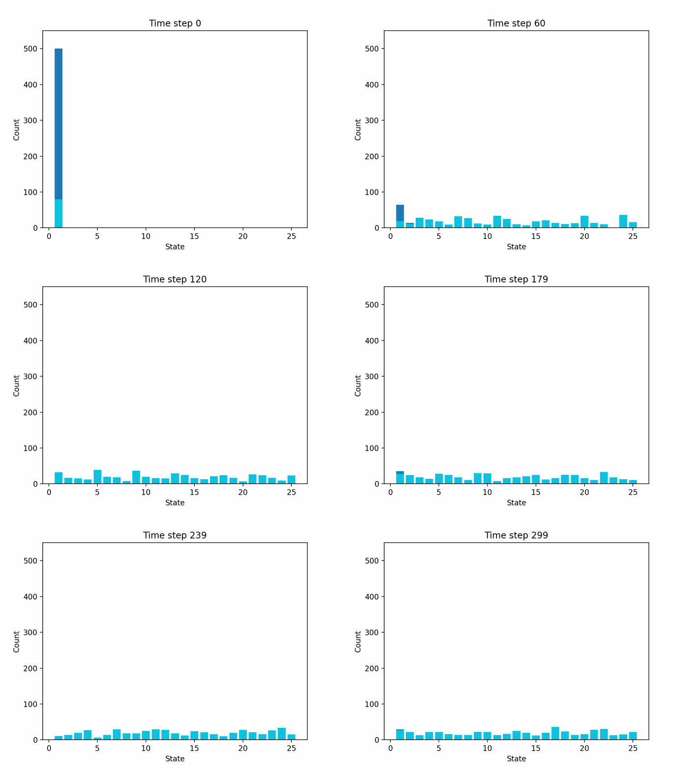
This approach turns out to work. As shown in Figure 11 below, the state distribution of the arms gradually converges to the uniform distribution, after which most arms continuously pass the episodes without triggering many failure events. Quantitatively, the average reward is about \(0.0774\) after simulating \(10^4\) time steps, close to the upper bound \(R_1^{\bar{\pi}^*} = 0.08\).

Recipe summary. To build a good policy for any restless bandit instance, follow two steps: (1) find the best policy for a single arm subject to a long-run budget constraint (i.e., the arm is active at most \(\alpha\) fraction of the time on average); (2) at each time step, let every arm independently decide whether it wants to be active according to this single-arm policy, and whenever more than \(\alpha N\) arms want to be active, fulfill as many requests as possible by prioritizing arms with smaller IDs. Together, these two steps yield the ID policy, which has a provable near-optimality guarantee on a broad class of instances — as we will state precisely in the next section.

Optimality Result

To state our main result, we first define some notation. Consider the Markov chain on the state space \(\mathbb{S}\) induced by the policy \(\bar{\pi}^*\). We let \(\mu^*\) be the stationary distribution of this Markov chain, and let \(P^t(s,s')\) be the \(t\)-step transition matrix. We define the mixing time \(\tau\) of this Markov chain as \[ \tau \triangleq \max_{s\in\mathbb{S}} \min \left\{t=0,1,2\dots \colon \sum_{s'\in\mathbb{S}} \left|P^t(s,s') - \mu^*(s') \right| \leq \frac{1}{e} \right\}. \] Intuitively, given any initial state \(s\in\mathbb{S}\), after \(\tau\) time steps, the state distribution of the Markov chain \(P^t(s,\cdot)\) is sufficiently close to the stationary distribution \(\mu^*(\cdot)\).

Theorem 1 : Assume \(\tau < \infty\), and let \(\pi\) be the ID policy. Then

$$ R_1^{\bar{\pi}^*} - R_N^\pi = O\left(\frac{\tau^4}{\sqrt{N}}\right), $$ where the constant factor in the big-O notation involves the parameters \(|\mathbb{S}|\), \(\alpha\), and \(\max_{s,a} |r(s,a)|\).

Remark : The mixing time assumption says that when an arm follows \(\bar{\pi}^*\), its state converges to the stationary distribution \(\mu^*\) within \(\tau\) time steps, regardless of where it started. In other words, \(\bar{\pi}^*\) randomizes the arm’s state in \(\tau\) steps, pulling it away from any bad initial state and making the states of different arms effectively independent. This independence enables a multiplexing effect, preventing the situation where a lot of arms need to be active simultaneously.

For the Flappy Bird example, under \(\bar{\pi}^*\), the bird always successfully passes every pipe, and then randomly transitions to a new episode that is HARD or EASY with equal probability. When the lengths of HARD and EASY episodes are relatively prime, the bird’s location after a sufficiently long time becomes uniform over all states, implying mixing.

Proof idea of Theorem 1:

One might wonder why this simple ID-based tie-breaking works. As discussed in Section 3 , this boils down to proving that after a certain period of time, all but an \(o(1)\) fraction of arms could follow the ideal actions sampled from \(\bar{\pi}^*\).
Here is the intuitive argument:

1. First, since we can activate at most \(\alpha N\) arms, \(\alpha N\) arms with the smallest IDs always follow \(\bar{\pi}^*\) under the ID policy.

2. These \(\alpha N\) arms will mix to the stationary distribution \(\mu^*\) after some time. After the mixing, the state of each arm is approximately an independent sample from \(\mu^*\), and requires activation with probability \(\alpha\). Consequently, the budget requirements of these \(\alpha N\) arms concentrate around \(\alpha * \alpha N = \alpha^2 N\).

   • Specializing to the Flappy Bird example, the states of the \(\alpha N\) arms converge to the uniform distribution, after which only about \(\alpha^2 N\) of them require focus.

3. Now consider the remaining \((1-\alpha)N\) arms: we can activate about \(\alpha N - \alpha^2 N = \alpha (1-\alpha) N\) of them, i.e., an \(\alpha\) fraction of the remaining arms. Repeating the argument in Step 2, the states of these arms will also mix to \(\mu^*\) after some time.

4. Repeating this process, the number of remaining arms not following \(\mu^*\) shrinks by approximately a factor of \((1-\alpha)\) per phase. In the long run, all but an \(o(1)\) fraction of arms could follow \(\bar{\pi}^*\), where the \(o(1)\) error terms come from the randomness in the budget requirements of the arms that have mixed.

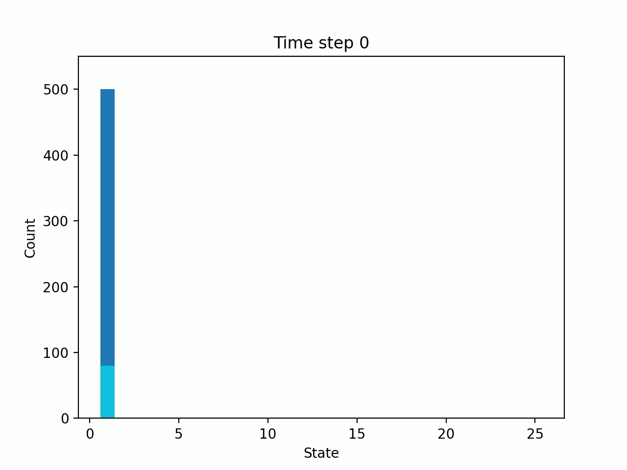
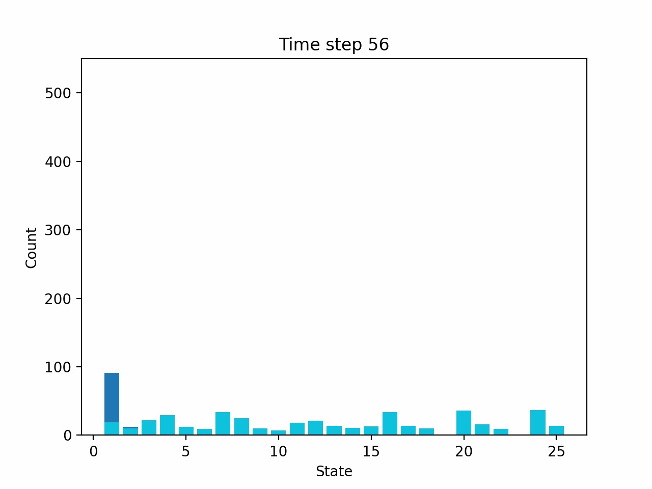
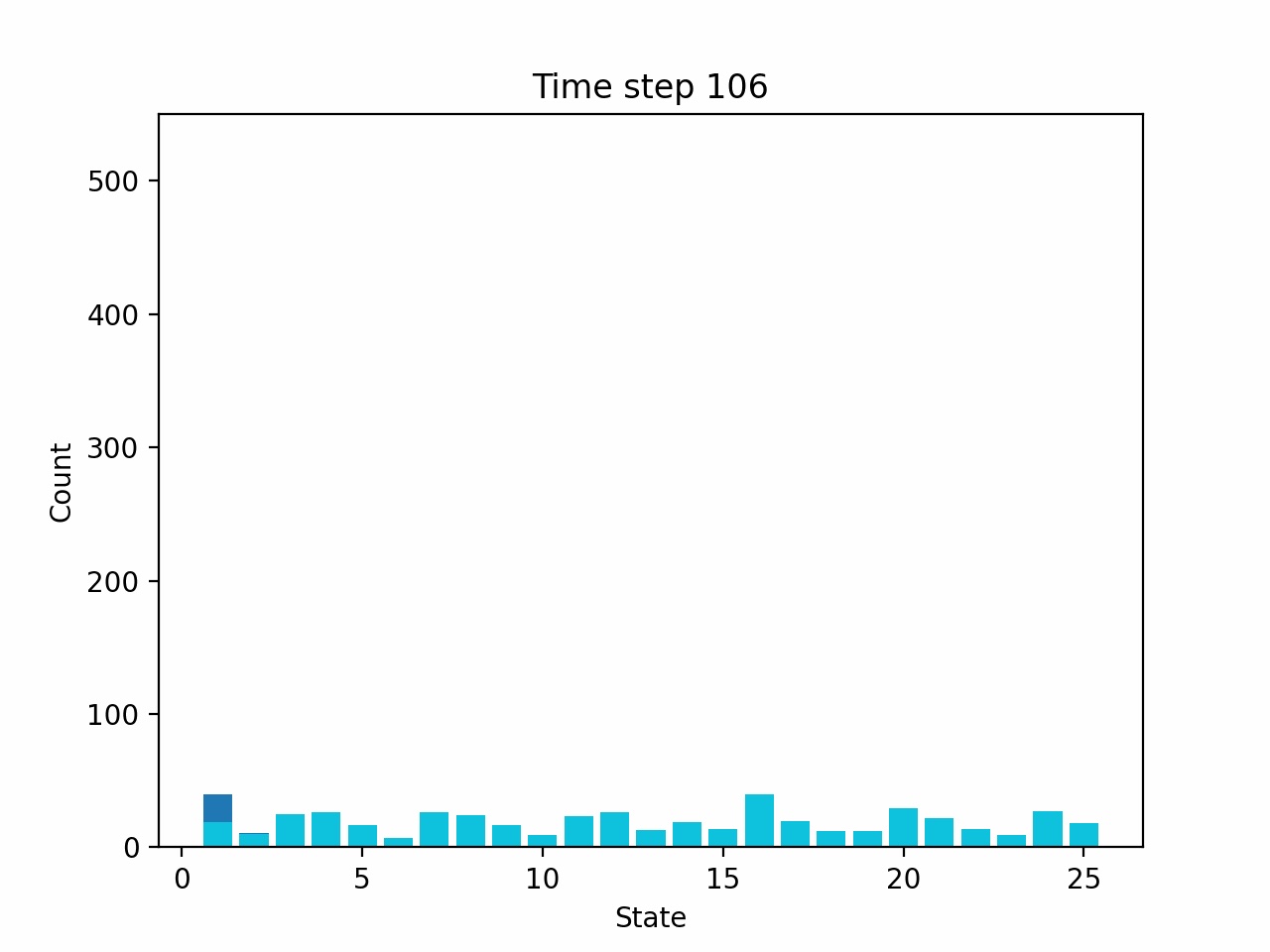
The process described above is illustrated in Figure 12 : from time step \(0\) to \(56\) to \(106\), more and more arms start to follow \(\bar{\pi}^*\) (cyan parts of the bars), and their empirical state distribution approaches the uniform distribution.

This multi-phase argument covers the main intuition behind the proof, except that in the rigorous proof, the mixing of the individual arms under \(\bar{\pi}^*\) and the expansion of the set of arms following \(\bar{\pi}^*\) happen simultaneously and continuously. To make an analogy, imagine a glacier melting from the bottom and gradually reducing to sea level ; the part of the glacier that begins to melt corresponds to the arms that start to follow \(\bar{\pi}^*\), whereas the part that has already melted corresponds to arms that have mixed to the uniform distribution. To track these two simultaneous changes and account for the occasional stochasticity that disrupts the convergence, we invent a technique called bivariate Lyapunov function .

We refer the readers to Section 5 of our paper for the details of this technique.

Generalizations

The techniques outlined in this blog could generalize beyond the restless bandit setting in multiple ways:

• We could allow multiple actions per arm. For the Flappy Bird example, this could mean having multiple levels of focus, each with a different success rate, and the total amount of focus that Sakiko could spend at any moment is subject to an upper limit.
  • We could even have a more refined model to control Sakiko’s specific movements when playing the game, such as tapping the game screen at a certain rate and pressure; different movements could lead to different outcomes, and require different amounts of focus. The total focus at any moment should be bounded by a fixed amount.
• We could also have multiple constraints. For the Flappy Bird example, this could mean each action is associated with two different types of costs, such as mental effort and physical effort; the total mental and physical efforts are subject to two separate constraints.
• We could also allow the arms to be heterogeneous, i.e., having different reward functions, transition dynamics, and cost functions for different arms. For the Flappy Bird example, different parallel sessions could have different success rates under the same actions.

The multi-action, multi-constraint generalization of restless bandits is called weakly-coupled Markov Decision Processes (WCMDPs). The policy design for WCMDPs follows the same idea described in this blog: first, consider a relaxation that decouples the controls of \(N\) arms into separate single-armed problems; second, convert the single-armed solution back to an \(N\)-armed policy using ID-based prioritization. The \(O(1/\sqrt{N})\) suboptimality gap can be proved almost verbatim, as the primary argument we use here is just the mixing of Markov chains.

With heterogeneity, the solution is more complex: for policy design, we need to uniformly shuffle the arms at time \(0\) before applying the ID policy, in case the low-ID arms happen to be “resource-hungry” and cause the high-ID arms to starve. The analysis is complicated by the fact that the empirical state distribution that we plot in Figures 10–12 no longer fully captures the system state, given the heterogeneity of the arms. We refer the readers to our second paper Projection-based Lyapunov method for fully heterogeneous weakly-coupled MDPs for more details.