We implemented the algorithm described in the last section in the same
LISP environment as the noise-free algorithms. The noise-tolerant
learning algorithm used was I-RIP, a separate-and-conquer
learner halfway between I-REP [32,30] and RIPPER
[14]. Like I-REP, it learns single rules by greedily adding
one condition at a time (using FOIL's information gain heuristic
[52]) until the rule no longer makes incorrect predictions on
the growing set, a randomly chosen set of 2/3 of the training
examples. Thereafter, the learned rule is simplified by greedily
deleting conditions as long as the performance of the rule does not
decrease on the remaining set of examples (the pruning set). All
examples covered by the resulting rule are then removed from the
training set and a new rule is learned in the same way until all
positive examples are covered by at least one rule or the stopping
criterion fires. Like RIPPER, I-RIP evaluates the quality of a rule
on the pruning set by computing the heuristic
![]() (where
p and n are the covered positive and negative examples
respectively) and stops adding rules to the theory whenever the
fraction of positive examples that are covered by the best rule does
not exceed 0.5. These choices have been shown to outperform I-REP's
original choices [14]. I-RIP is quite similar to I-REP*,
which is also described by [14], but it retains I-REP's
method of considering all conditions for pruning (instead of
considering a final sequence of conditions).
(where
p and n are the covered positive and negative examples
respectively) and stops adding rules to the theory whenever the
fraction of positive examples that are covered by the best rule does
not exceed 0.5. These choices have been shown to outperform I-REP's
original choices [14]. I-RIP is quite similar to I-REP*,
which is also described by [14], but it retains I-REP's
method of considering all conditions for pruning (instead of
considering a final sequence of conditions).
Around I-RIP, we wrapped the windowing procedure of Figure 9. The resulting algorithm is referred to as WIN-RIP-NT.15 Again, the implementations of both algorithms remove semantically redundant rules in a post-processing phase as described in section 4.2.
We studied the behavior of the algorithms in the KRK illegality domain with varying levels of artificial noise. A noise level of n% means that in about n% of the examples the class label has been replaced with a random class label. In each of the experiments described in this section, we report the average results on 10 different subsets in terms of run-time of the algorithm and measured accuracy on a separate noise-free test set. We did not evaluate the algorithms according to the total number of examples processed by the basic learning algorithm, because the way we compute the completeness check (doubling the size of the window if no rules can be learned from the current window, see section 5.2.2) makes these results less useful. All algorithms were run on identical data sets, but some random variation results from the fact that I-RIP uses internal random splits of the training data. All experiments shown below were conducted with the same parameter setting of InitSize = 100and MaxIncSize = 50 which performed well in the noise-free case. We have not yet made an attempt to evaluate their appropriateness for noisy domains.
First, we aimed at making sure that the noise-free setting (
![]() )
of the WIN-RIP-NT algorithm still performs reasonably
well, so that the noise-tolerant generalization of the
INTEGRATIVEWINDOWING algorithm does not lose its efficiency in
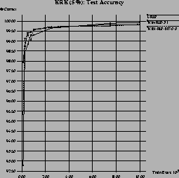
noise-free domains. Figure 10 shows the performance of
I-RIP, WIN-RIP-3.1 (basic windowing using I-RIP in its loop),
WIN-RIP-95 (integrative windowing using I-RIP), and
WIN-RIP-NT-0.0 (the noise-tolerant version of integrative windowing
with a setting of
)
of the WIN-RIP-NT algorithm still performs reasonably
well, so that the noise-tolerant generalization of the
INTEGRATIVEWINDOWING algorithm does not lose its efficiency in
noise-free domains. Figure 10 shows the performance of
I-RIP, WIN-RIP-3.1 (basic windowing using I-RIP in its loop),
WIN-RIP-95 (integrative windowing using I-RIP), and
WIN-RIP-NT-0.0 (the noise-tolerant version of integrative windowing
with a setting of
![]() ). The graphs resemble very much the
graphs of Figure 5 for the KRK domain, except that
I-RIP over-generalizes occasionally, so that the accuracy never
reaches exactly 100%. WIN-RIP-NT-0.0 performs a little worse
than WIN-RIP-95, but it still is better than regular
windowing. A similar graph for the Mushroom domain is shown in
previous work [29]. So we can conclude that the changes in
the algorithm did some harm, but the algorithm still performs
reasonably well in noise-free domains.
). The graphs resemble very much the
graphs of Figure 5 for the KRK domain, except that
I-RIP over-generalizes occasionally, so that the accuracy never
reaches exactly 100%. WIN-RIP-NT-0.0 performs a little worse
than WIN-RIP-95, but it still is better than regular
windowing. A similar graph for the Mushroom domain is shown in
previous work [29]. So we can conclude that the changes in
the algorithm did some harm, but the algorithm still performs
reasonably well in noise-free domains.

 |
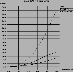
Figure 11 shows the performance of three of these algorithms (we did not test WIN-RIP-95) for datasets with 5% artificial noise. Here, I-RIP is clearly the fastest algorithm, a windowed version takes about twice as long. Although this is only a moderate level of noise, integrative windowing with WIN-RIP-NT-0.0 is already unacceptably slow because it successively adds all examples into the window as we have discussed in section 5.2.1.
The interesting question, of course, is what happens if we increase
the ![]() parameter, which supposedly should be able to deal with
the noise in the data? To this end, we have performed a series of
experiments with varying noise and varying values for the
parameter, which supposedly should be able to deal with
the noise in the data? To this end, we have performed a series of
experiments with varying noise and varying values for the ![]() parameters. Our basic finding is that the algorithm is very sensitive
to the choice of the
parameters. Our basic finding is that the algorithm is very sensitive
to the choice of the ![]() -parameter. The first thing to notice is
that there is an inverse relationship between the
-parameter. The first thing to notice is
that there is an inverse relationship between the ![]() -value and
the run-time of the algorithm. This is not surprising because higher
values of
-value and
the run-time of the algorithm. This is not surprising because higher
values of ![]() will make it easier for rules to be added to the
final theory. Thus, the algorithm is likely to terminate earlier.
On the other hand, we also notice a correlation between predictive
accuracy and the value of
will make it easier for rules to be added to the
final theory. Thus, the algorithm is likely to terminate earlier.
On the other hand, we also notice a correlation between predictive
accuracy and the value of ![]() .
The reason for this is that lower
.
The reason for this is that lower
![]() -values impose more stringent restrictions on the quality of
the accepted rules. Again, this can be explained with the fact that
higher
-values impose more stringent restrictions on the quality of
the accepted rules. Again, this can be explained with the fact that
higher ![]() values are likely to admit less accurate rules (see
section 5.2.1).
values are likely to admit less accurate rules (see
section 5.2.1).
Therefore, what we hope to find, is an ``optimal'' range for the
![]() -parameter for which WIN-RIP-NT- outperforms
I-RIP in terms of run-time while maintaining about the same
performance in terms of accuracy. For example,
Figure 12 shows the results of I-RIP and
WIN-RIP-NT with a setting of
-parameter for which WIN-RIP-NT- outperforms
I-RIP in terms of run-time while maintaining about the same
performance in terms of accuracy. For example,
Figure 12 shows the results of I-RIP and
WIN-RIP-NT with a setting of
![]() in the KRK domain with
20% noise added. Both perform about the same in terms of accuracy,
but there is some gain in terms of run-time. Although it is not as
remarkable as in noise-free domains, there is a clear difference in
the growth function: I-RIP's run-time grows faster with increasing
sample set sizes, while WIN-RIP-NT's growth function appears to
be sub-linear.
Unfortunately, the performance of the algorithm seems to be quite
sensitive to the choice of
in the KRK domain with
20% noise added. Both perform about the same in terms of accuracy,
but there is some gain in terms of run-time. Although it is not as
remarkable as in noise-free domains, there is a clear difference in
the growth function: I-RIP's run-time grows faster with increasing
sample set sizes, while WIN-RIP-NT's growth function appears to
be sub-linear.
Unfortunately, the performance of the algorithm seems to be quite
sensitive to the choice of ![]() ,
so that we cannot give a general
recommendation for a setting for
,
so that we cannot give a general
recommendation for a setting for ![]() .16 Figure 13 shows the graph for three
different settings of the
.16 Figure 13 shows the graph for three
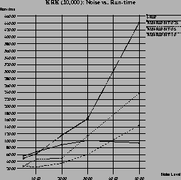
different settings of the ![]() -parameter for varying levels of
noise. In terms of run-time, it is obvious that higher values of
-parameter for varying levels of
noise. In terms of run-time, it is obvious that higher values of
![]() produce lower run-times. In terms of accuracy,
produce lower run-times. In terms of accuracy,
![]() seems to be a consistently good choice. However, for example, at a
noise level of 30%
the version with
seems to be a consistently good choice. However, for example, at a
noise level of 30%
the version with
![]() is clearly
preferable when considering the performance in both dimensions. With
further increasing noise levels, all algorithms become prohibitively
expensive, but are able to achieve surprisingly good results in terms
of accuracy. From this and similar experiments, we conclude that there
seems to be some correlation between an optimal choice of the
is clearly
preferable when considering the performance in both dimensions. With
further increasing noise levels, all algorithms become prohibitively
expensive, but are able to achieve surprisingly good results in terms
of accuracy. From this and similar experiments, we conclude that there
seems to be some correlation between an optimal choice of the
![]() -parameter and the noise-level in the data.
-parameter and the noise-level in the data.

 |
We have also tested WIN-RIP-NT on a discretized, 2-class version of Quinlan's 9172 example thyroid diseases database, where we achieved improvements in terms of both, run-time and accuracy with the windowing algorithms. These experiments are discussed in previous work [29]. However, later experiments showed that this domain exhibited the same kind of behavior as the Shuttle domain, shown in Figure 7, i.e., most versions of WIN-RIP-NT consistently outperformed I-RIP in terms of accuracy when learning on the minority class, while this picture reversed when learning on the majority class. Run-time gains could be observed in both cases. However, these results can only be regarded as preliminary. In order to answer the question whether our results in the KRK domain with artificial class noise are predictive for the algorithm's performance on real-world problems, a more elaborate study must be performed.
In summary, we have discussed why noisy data appear to be a problem for windowing algorithms and have argued that three basic problems have to be addressed in order to adapt windowing to noisy domains. We have also shown that, with three particular choices for these procedures, it is in fact possible to achieve run-time gains without sacrificing accuracy. However, we do not claim that these three particular choices are optimal and are convinced that better choices are possible and should lead to a more robust learning system.