Exponential Family PCA

The conventional view of PCA is a geometric one, finding a low-dimensional projection that minimizes the squared-error loss. An alternate view is a probabilistic one: if the data consist of samples drawn from a probability distribution, then PCA is an algorithm for finding the parameters of the generative distribution that maximize the likelihood of the data. The squared-error loss function corresponds to an assumption that the data is generated from a Gaussian distribution. Collins, Dasgupta & Schapire [CDS02] demonstrated that PCA can be generalized to a range of loss functions by modeling the data with different exponential families of probability distributions such as Gaussian, binomial, or Poisson. Each such exponential family distribution corresponds to a different loss function for a variant of PCA, and Collins, Dasgupta & Schapire [CDS02] refer to the generalization of PCA to arbitrary exponential family data-likelihood models as ``Exponential family PCA'' or E-PCA.

An E-PCA model represents the reconstructed data using a low-dimensional weight vector $\tilde b$, a basis matrix $U$, and a link function $f$:

$$b\approx f(U\tilde b)$$ (4)

Each E-PCA model uses a different link function, which can be derived from its data likelihood model (and its corresponding error distribution and loss function). The link function is a mapping from the data space to another space in which the data can be linearly represented.

The link function $f$ is the mechanism through which E-PCA generalizes dimensionality reduction to non-linear models. For example, the identity link function corresponds to Gaussian errors and reduces E-PCA to regular PCA, while the sigmoid link function corresponds to Bernoulli errors and produces a kind of ``logistic PCA'' for 0-1 valued data. Other nonlinear link functions correspond to other non-Gaussian exponential families of distributions.

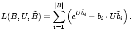
We can find the parameters of an E-PCA model by maximizing the log-likelihood of the data under the model, which has been shown [CDS02] to be equivalent to minimizing a generalized Bregman divergence

$$B_{F^*}(b \Vert U\tilde{b} ) = F(U\tilde{b}) - b\cdot U\tilde{b} + F^*(b)$$ (5)

between the low-dimensional and high-dimensional representations, which we can solve using convex optimization techniques. (Here $F$ is a convex function whose derivative is $f$, while $F^*$ is the convex dual of $F$. We can ignore $F^*$ for the purpose of minimizing equation 5 since the value of $b$ is fixed.) The relationship between PCA and E-PCA through link functions is reminiscent of the relationship between linear regression and Generalized Linear Models [MN83].

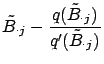
To apply E-PCA to belief compression, we need to choose a link function which accurately reflects the fact that our beliefs are probability distributions. If we choose the link function

$$f(U\tilde b) = e^{U\tilde b}$$ (6)

then it is not hard to verify that $F(U\tilde b) = \sum e^{U\tilde b}$ and $F^*(b)=b\cdot\ln b-\sum b$. So, equation 5 becomes

$$B_{F^*}(b \Vert U\tilde{b} ) = \sum e^{U\tilde{b}} - b\cdot U\tilde{b} + b\cdot\ln b - \sum b$$ (7)

If we write $\hat b = f(U\tilde b)$, then equation 7 becomes

$$B_{F^*}(b \Vert U\tilde{b} ) = b \cdot \ln b - b \cdot \ln \hat b + \sum \hat b - \sum b = UKL(b \Vert \hat{b} )$$

where $UKL$ is the unnormalized KL divergence. Thus, choosing the exponential link function (6) corresponds to minimizing the unnormalized KL divergence between the original belief and its reconstruction. This loss function is an intuitively reasonable choice for measuring the error in reconstructing a probability distribution.⁵ The exponential link function corresponds to a Poisson error model for each component of the reconstructed belief.

Our choice of loss and link functions has two advantages: first, the exponential link function constrains our low-dimensional representation $e^{U\tilde{b}}$ to be positive. Second, our error model predicts that the variance of each belief component is proportional to its expected value. Since PCA makes significant errors close to 0, we wish to increase the penalty for errors in small probabilities, and this error model accomplishes that.

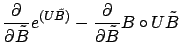
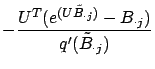
If we compute the loss for all $b_i$, ignoring terms that depend only on the data $b$, then⁶

$$L(B, U, \tilde{B}) = \sum_{i=1}^{\vert B\vert} \left ( e^{U\tilde{b}_i} - b_i \cdot U\tilde{b}_i \right ).$$ (8)

The introduction of the link function raises a question: instead of using the complex machinery of E-PCA, could we just choose some non-linear function to project the data into a space where it is linear, and then use conventional PCA? The difficulty with this approach is of course identifying that function; in general, good link functions for E-PCA are not related to good nonlinear functions for application before regular PCA. So, while it might appear reasonable to use PCA to find a low-dimensional representation of the log beliefs, rather than use E-PCA with an exponential link function to find a representation of the beliefs directly, this approach performs poorly because the surface is only locally well-approximated by a log projection. E-PCA can be viewed as minimizing a weighted least-squares that chooses the distance metric to be appropriately local. Using conventional PCA over log beliefs also performs poorly in situations where the beliefs contain extremely small or zero probability entries.

Finding the E-PCA Parameters

Algorithms for conventional PCA are guaranteed to converge to a unique answer independent of initialization. In general, E-PCA does not have this property: the loss function (8) may have multiple distinct local minima. However, the problem of finding the best $\tilde B$ given $B$ and $U$ is convex; convex optimization problems are well studied and have unique global solutions [Roc70]. Similarly, the problem of finding the best $U$ given $B$ and $\tilde B$ is convex. So, the possible local minima in the joint space of $U$ and $\tilde B$ are highly constrained, and finding $U$ and $\tilde B$ does not require solving a general non-convex optimization problem.

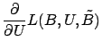
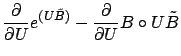
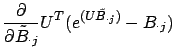
Gordon [Gor03] describes a fast, Newton's Method approach for computing $U$ and $\tilde{B}$ which we summarize here. This algorithm is related to Iteratively Reweighted Least Squares, a popular algorithm for generalized linear regression [MN83]. In order to use Newton's Method to minimize equation (8), we need its derivative with respect to $U$ and $\tilde{B}$:

$$\frac{\partial}{\partial U} L(B, U, \tilde{B}) = \frac{\partial}{\partial U} e^{(U\tilde{B})} - \frac{\partial}{\partial U} B \circ U\tilde{B}$$ (9)

$$= e^{(U\tilde{B})} \tilde{B}^T - B \tilde{B}^T$$ (10)

$$= (e^{(U\tilde{B})} - B ) \tilde{B}^T$$ (11)

and

$$\frac{\partial}{\partial \tilde{B}} L(B, U, \tilde{B}) = \frac{\partial}{\partial \tilde{B}} e^{(U\tilde{B})} - \frac{\partial}{\partial \tilde{B}} B \circ U\tilde{B}$$ (12)

$$= U^T e^{(U\tilde{B})} - U^T B$$ (13)

$$= U^T (e^{(U\tilde{B})} - B).$$ (14)

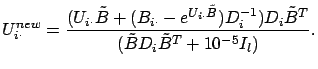
If we set the right hand side of equation (14) to zero, we can iteratively compute $\tilde{B}_{\cdot j}$, the $j^{th}$ column of $\tilde{B}$, by Newton's method. Let us set $q(\tilde{B}_{\cdot j}) = U^T(e^{(U\tilde{B}_{\cdot j})}-B_{\cdot j})$, and linearize about $\tilde{B}_{\cdot j}$ to find roots of $q()$. This gives

$$\tilde{B}^{new}_{\cdot j} = \tilde{B}_{\cdot j} - \frac{q(\tilde{B}_{\cdot j})}{q'(\tilde{B}_{\cdot j})}$$ (15)

$$\tilde{B}^{new}_{\cdot j} - \tilde{B}_{\cdot j} = - \frac{U^T (e^{(U\tilde{B}_{\cdot j})} - B_{\cdot j})} {q'(\tilde{B}_{\cdot j})}$$ (16)

Note that equation 15 is a formulation of Newton's method for finding roots of $q$, typically written as

$$x_{n+1} = x_n - \frac{f(x_n)}{f'(x_n)}.$$ (17)

We need an expression for $q'$:

$$\frac{\partial q}{\partial \tilde{B}_{\cdot j}} = \frac{\partial }{\partial \tilde{B}_{\cdot j}}U^T (e^{(U\tilde{B}_{\cdot j})} - B_{\cdot j})$$ (18)

$$= \frac{\partial }{\partial \tilde{B}_{\cdot j}}U^T e^{(U\tilde{B}_{\cdot j})}$$ (19)

$$= U^T D_j U$$ (20)

We define $D_j$ in terms of the $\mathtt{diag}$ operator that returns a diagonal matrix:

$$D_j = \mathtt{diag}(e^{U \tilde{B}_{\cdot j}}),$$ (21)

where

$$\mathtt{diag}(b) = \begin{bmatrix}b(s_0) & \ldots & 0 \vdots & \ddots & \vdots 0 & \ldots & b(s_{\vert\mathcal{S}\vert}) \end{bmatrix}.$$ (22)

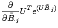
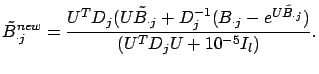
Combining equation (15) and equation (20), we get

$$(U^T D_j U) (\tilde{B}^{new}_{\cdot j} - \tilde{B}_{\cdot j}) = U^T (B_{\cdot j} - e^{U\tilde{B}_{\cdot j}})$$ (23)

$$U^T D_j U \tilde{B}^{new}_{\cdot j} = (U^T D_j U) \tilde{B}_{\cdot j} + U^T D_j D_j^{-1} (B_{\cdot j} - e^{U\tilde{B}_{\cdot j}})$$ (24)

$$= U^T D_j (U \tilde{B}_{\cdot j} + D_j^{-1} (B_{\cdot j} - e^{U\tilde{B}_{\cdot j}}),$$ (25)

which is a weighted least-squares problem that can be solved with standard linear algebra techniques. In order to ensure that the solution is numerically well-conditioned, we typically add a regularizer to the divisor, as in

$$\tilde{B}^{new}_{\cdot j} = \frac{U^T D_j (U \tilde{B}_{\cdot j} + D_j^{-1} (B_{\cdot j} - e^{U\tilde{B}_{\cdot j}})}{(U^T D_j U + 10^{-5}I_l)}.$$ (26)

where $I_l$ is the $l \times l$ identity matrix. Similarly, we can compute a new $U$ by computing $U_{i \cdot}$, the $i^{th}$ row of $U$, as

$$U^{new}_{i \cdot} = \frac{(U_{i \cdot} \tilde{B} + (B_{i \cdot} -... ...tilde{B}})D_i^{-1}) D_i \tilde{B}^T}{(\tilde{B} D_i \tilde{B}^T + 10^{-5}I_l)}.$$ (27)

The E-PCA Algorithm

We now have an algorithm for automatically finding a good low-dimensional representation $\tilde{\mathbb{B}}$ for the high-dimensional belief set $\mathbb{B}$. This algorithm is given in Table 1; the optimization is iterated until some termination condition is reached, such as a finite number of iterations, or when some minimum error $\epsilon$ is achieved.

1. Collect a set of sample beliefs from the high-dimensional belief space
2. Assemble the samples into the data matrix $B = [ b_1 \vert \ldots \vert b_{\vert B\vert} ]$
3. Choose an appropriate loss function, $L(B, U, \tilde{B})$
4. Fix an initial estimate for $\tilde{B}$ and $U$ randomly
5. do
6. For each column $\tilde{B}_{\cdot j} \in \tilde{B}$,
7. Compute $\tilde{B}_{\cdot j}^{new}$ using current $U$ estimate from equation (26)
8. For each row $U_{i \cdot} \in U$,
9. Compute $U_{i \cdot}^{new}$ using new $\tilde{B}$ estimate from equation (27)
10. while $L(B, U, \tilde{B}) > \epsilon$

Table 1: The E-PCA Algorithm for finding a low-dimensional representation of a POMDP, including Gordon's Newton's method [Gor03].

The steps 7 and 9 raise one issue. Although solving for each row of $U$ or column of $\tilde{B}$ separately is a convex optimization problem, solving for the two matrices simultaneously is not. We are therefore subject to potential local minima; in our experiments we did not find this to be a problem, but we expect that we will need to find ways to address the local minimum problem in order to scale to even more complicated domains.

Once the bases $U$ are found, finding the low-dimensional representation of a high-dimensional belief is a convex problem; we can compute the best answer by iterating equation (26). Recovering a full-dimensional belief $b$ from the low-dimensional representation $\tilde{b}$ is also very straightforward:

$$x = e^{U\tilde{b}}.$$ (28)

Our definition of PCA does not explicitly factor the data into $U$, $S$ and $\tilde{B}$ as many presentations do. In this three-part representation of PCA, $S$ contains the singular values of the decomposition, and $U$ and $\tilde B$ are orthonormal. We use the two-part representation $B\approx f(U\tilde B)$ because there is no quantity in the E-PCA decomposition which corresponds to the singular values in PCA. As a result, $U$ and $\tilde B$ will not in general be orthonormal. If desired, though, it is possible to orthonormalize $U$ as an additional step after optimization using conventional PCA and adjust $\tilde B$ accordingly.

Footnotes

... distribution.⁵

If we had chosen the link function $e^{U\tilde b}/\sum e^{U\tilde b}$ we would have arrived at the normalized KL divergence, which is perhaps an even more intuitively reasonable way to measure the error in reconstructing a probability distribution. This more-complicated link function would have made it more difficult to derive the Newton equations in the following pages, but not impossible; we have experimented with the resulting algorithm and found that it produces qualitatively similar results to the algorithm described here. Using the normalized KL divergence does have one advantage: it can allow us to get away with one fewer basis function during planning, since for unnormalized KL divergence the E-PCA optimization must learn a basis which can explicitly represent the normalization constant.

... then⁶

E-PCA is related to Lee and Seung's [LS99] non-negative matrix factorization. One of the NMF loss functions presented by Lee & Seung [LS99] penalizes the KL-divergence between a matrix and its reconstruction, as we do in equation 8; but, the NMF loss does not incorporate a link function and so is not an E-PCA loss. Another NMF loss function presented by Lee & Seung [LS99] penalizes squared error but constrains the factors to be nonnegative; the resulting model is an example of a (GL)$^2$M, a generalization of E-PCA described by Gordon [Gor03].