What Bounds Can Learn From Each Other

Consider a Markov network defined by the potentials $\psi_{i}\left(S_{i}\right)$ each dependent on a set of nodes $S_{i}$. The probability to find the network in a certain state $S$ is proportional to

$$p\left(S\right)\propto\prod_i\psi_{i}\left(S_{i}\right)$$ (1)

Problems arise when one is interested in the marginal probability over a small number of nodes (denoted by $S_\mathrm{\scriptscriptstyle mar}$), since in general this requires the summation over all of the exponentially many states.

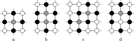
Figure: Examples of separator and marginal nodes in an (infinite) Ising grid. Light shaded nodes correspond to $S_\mathrm{\scriptscriptstyle mar}$, black nodes to $S_\mathrm{\scriptscriptstyle sep}$. (a) A single node enclosed by its tightest separator. (b), (c) Two marginal nodes enclosed by their tightest separator. (d) Another choice for a separator for a single node marginal; the other node enclosed by that separator belongs to $S_\mathrm{\scriptscriptstyle oth}$.

Let us define the set of separator nodes, $S_\mathrm{\scriptscriptstyle sep}$, to be the nodes that separate $S_\mathrm{\scriptscriptstyle mar}$ from the rest of the network. One can take, for instance, the union of the nodes in all potentials that contain at least one marginal node, while excluding the marginal nodes itself in that union (which is the Markov blanket of $S_\mathrm{\scriptscriptstyle mar}$):

$$S_\mathrm{\scriptscriptstyle sep}=\bigcup_{S_{i}\cap S_\math... ...}\neq\emptyset} \!\!\!S_{i}/S_\mathrm{\scriptscriptstyle mar}$$ (2)

See for instance Figure a-c. It is not necessary, however, that $S_\mathrm{\scriptscriptstyle sep}$ defines a tight separation. There can be a small number of other nodes, $S_\mathrm{\scriptscriptstyle oth}$, inside the separated area, but not included by $S_\mathrm{\scriptscriptstyle mar}$ (Figure d). A sufficient condition for the rest of the theory is that the size of the total state space, $\left\Vert S_\mathrm{\scriptscriptstyle sep}\cup S_\mathrm{\scriptscriptstyle mar}\cup S_\mathrm{\scriptscriptstyle oth}\right\Vert$, is small enough to do exact computations.

Suppose that we know a particular setting of the separator nodes, $\vec s_\mathrm{\scriptscriptstyle sep}$, then computing the conditional distribution of $S_\mathrm{\scriptscriptstyle mar}$ given $S_\mathrm{\scriptscriptstyle sep}$ is easy:

$$p\left(\vec s_\mathrm{\scriptscriptstyle mar} \vert \vec s... ...yle oth} \vert \vec s_\mathrm{\scriptscriptstyle sep}\right)$$ (3)

This expression is tractable to compute since $S_\mathrm{\scriptscriptstyle sep}$ serves as the Markov blanket for the union of $S_\mathrm{\scriptscriptstyle mar}$ and $S_\mathrm{\scriptscriptstyle oth}$. Thus the actual numbers are independent of the rest of the network and can be found either by explicitly doing the summation or by any other more sophisticated method. Similarly, if we would know the exact distribution over the separator nodes, we can easily compute the marginal probability of $S_\mathrm{\scriptscriptstyle mar}$:

$$p\left(\vec s_\mathrm{\scriptscriptstyle mar}\right)=\sum_{\... ...ep}\right)p\left(\vec s_\mathrm{\scriptscriptstyle sep}\right)$$ (4)

Unfortunately, in general we do not know the distribution $p\left(\vec s_\mathrm{\scriptscriptstyle sep}\right)$ and therefore we cannot compute $p\left(\vec s_\mathrm{\scriptscriptstyle mar}\right)$. We can, however, still derive certain properties of the marginal distribution, namely upper and lower bounds for each state of $S_\mathrm{\scriptscriptstyle mar}$. For instance, an upper bound on $\vec s_\mathrm{\scriptscriptstyle mar}$ can easily be found by computing

$$p_+\left(\vec s_\mathrm{\scriptscriptstyle mar}\right)=\math... ...ep}\right)q\left(\vec s_\mathrm{\scriptscriptstyle sep}\right)$$ (5)

under the constraints $\forall_{\vec s_\mathrm{\scriptscriptstyle sep}\in S_\mathrm{\scriptscriptstyle sep}}\;q\left(\vec s_\mathrm{\scriptscriptstyle sep}\right)\ge0$ and $\sum_{\vec s_\mathrm{\scriptscriptstyle sep}\in S_\mathrm{\scriptscriptstyle sep}}q\left(\vec s_\mathrm{\scriptscriptstyle sep}\right)=1$. The distribution $q\left(\vec s_\mathrm{\scriptscriptstyle sep}\right)$ corresponds to $\left\Vert S_\mathrm{\scriptscriptstyle sep}\right\Vert$ free parameters (under the given constraints) used to compute the worst case (here: the maximum) marginal value for each $\vec s_\mathrm{\scriptscriptstyle mar}$. Obviously, if $q\left(\vec s_\mathrm{\scriptscriptstyle sep}\right)=p\left(\vec s_\mathrm{\scriptscriptstyle sep}\right)$ the upper bound corresponds to the exact value, but in general $p\left(\vec s_\mathrm{\scriptscriptstyle sep}\right)$ is unknown and we have to maximize over all possible distributions. One may recognize Equation  as a simple linear programming (LP) problem with $\left\Vert S_\mathrm{\scriptscriptstyle sep}\right\Vert$ variables. With a similar equation we can find lower bounds $p_-\left(\vec s_\mathrm{\scriptscriptstyle mar}\right)$.

Upto now we did not include any information about $q\left(\vec s_\mathrm{\scriptscriptstyle sep}\right)$ we might have into the equation above. But suppose that we already computed upper and lower bounds on the marginals of other nodes than $S_\mathrm{\scriptscriptstyle mar}$. How can we make use of this knowledge? We investigate our table of all sets of marginal nodes we bounded earlier and take out those that are subsets of $S_\mathrm{\scriptscriptstyle sep}$. Obviously, whenever we find already computed bounds on $S_\mathrm{\scriptscriptstyle mar}'$ where $S_\mathrm{\scriptscriptstyle mar}'\subseteq S_\mathrm{\scriptscriptstyle sep}$¹, we can be sure that

$$\sum_{\vec s_\mathrm{\scriptscriptstyle sep}\in S_\mathrm{\s... ...makebox[0pt][l]{$ '$}}_\mathrm{\scriptscriptstyle mar}\right)$$ (6)

and similarly for the lower bound. These equations are nothing more than extra contraints on $q\left(\vec s_\mathrm{\scriptscriptstyle sep}\right)$ which we may include in the LP-problem in Equation . There can be several $S_\mathrm{\scriptscriptstyle mar}'$ that are subsets of $S_\mathrm{\scriptscriptstyle sep}$ each defining $2\left\Vert S_\mathrm{\scriptscriptstyle mar}'\right\Vert$ extra constraints.

In this way, information collected by bounds computed earlier, can propagate to $S_\mathrm{\scriptscriptstyle mar}$, thereby finding tighter bounds for these marginals. This process can be repeated for all sets of marginal nodes we have selected until convergence is reached.