Linear Programming

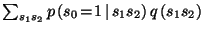
Figure: The area in which $q\left(s_1s_2\right)$ must lie is shown. $q\left(00\right)$ is implicitly given since the distribution is normalized. a) The pyramid is the allowable space. The darker planes show how this pyramid can be restricted by adding earlier computed bounds as constraints in the linear programming problem. b) This results in a smaller polyhedron. The black lines show the planes where the function $\sum_{s_1s_2}p\left(s_0\!=\!1 \vert s_1s_2\right)q\left(s_1s_2\right)$ is constant for this particular problem.

In terms of standard linear programming, Equation  can be expressed as

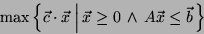$$\mathrm{max} \Big\{\vec c\cdot\vec x\:\Big\vert\: \vec x\ge0 \wedge A\vec x\le\vec b \Big\}$$ (7)

where the variables are defined as
$$\begin{align} \vec x&=q\left(\vec s_\mathrm{\scriptscriptstyle sep}\right) \\ \... ...scriptscriptstyle mar}\in S_\mathrm{\scriptscriptstyle mar}'}\right) \end{align}$$
where $\delta\left({\vec s\makebox[0pt][l]{$ '$}}_\mathrm{\scriptscriptstyle mar},\vec s_\mathrm{\scriptscriptstyle sep}\right)=1$ iff the states of the nodes both node sets have in common are equal. Thus the columns of the matrix $A$ correspond to $\vec s_\mathrm{\scriptscriptstyle sep}$, the rows of $A$ and $b$ to all the constraints (of which we have $2\left\Vert S_\mathrm{\scriptscriptstyle mar}'\right\Vert$ for each $S_\mathrm{\scriptscriptstyle mar}'\subseteq S_\mathrm{\scriptscriptstyle sep}$). The ordering of the rows of $A$ and $b$ is irrelevant as long as it is the same for both. The constraint that $q\left(\vec s_\mathrm{\scriptscriptstyle sep}\right)$ should be normalized can be incorporated in $A$ and $\vec b$ by requiring

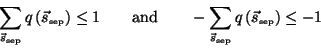$$\sum_{\vec s_\mathrm{\scriptscriptstyle sep}}q\left(\vec s_\... ...sep}}q\left(\vec s_\mathrm{\scriptscriptstyle sep}\right)\le-1$$ (8)

The maximum of $\vec c\cdot\vec x$ corresponds to $p_+\left(\vec s_\mathrm{\scriptscriptstyle mar}\right)$. The negative of $p_-\left(\vec s_\mathrm{\scriptscriptstyle mar}\right)$ can be found by using $-\vec c\cdot\vec x$ as the objective function.